Projecting future results – Skater edition

Abstract:

I have previously introduced the sGAA model (See here), which is primarily a descriptive model. Now I will introduce a predictive counterpart – projected sGAA or p-sGAA. It’s based on 3 years of weighted data.

sGAA describes past performances while p-sGAA projects future performances.

The projection model:

The model is basically based on 3 years weighted sGAA data (I will get back to this a little later). There’s nothing spectacular or innovative about this. Other player based projection models (like Dom Luszczyszyn’s model) are built in a similar way.

However, my model differs in two ways:

1. The baseline is league average and not replacement level. This makes the model easier to interpret, as one p-sGAA is worth one goal to the team’s goal differential. It also allows me to include all players (no minimum requirements) since a player with little or no NHL experience will be considered average by default.
2. The model uses total numbers instead of rates – it’s based on sGAA instead of sGAA per 60 minutes. This means that there’s no minimum TOI requirement and I don’t have to estimate the ice time/role of every player. The model assumes the role remains the same as it has been for the previous 3 years – It expects TOI to equal p-TOI.

Sometimes less is more. In this case the model structure is very simple. It’s just based on sGAA data. I prefer my model not to include any kind of subjective estimations. Is it perfect to assume every rookie is an average NHL’er? No… but using scouting reports isn’t perfect either. I want the model to be based on NHL data only.

Overall, I think it’s a good approach. If someone like Conor McDavid enters the league you will have to include that in your interpretation and analysis of the model.

No model will ever be perfect. It’s all about knowing how to interpret the model.

Weighing the data:

First step is to weigh the data. Obviously, the newest information holds the most importance and should be weighed accordingly.

I’ve tried a few different weighings to see when p-sGAA correlates best with sGAA. I found that the correlation was best with a weighing in between 3-2-1 and 4-3-2. So, here’s the calculated p-sGAA:

p-sGAA(Year_x) = (51/108) * sGAA(Year_x-1) + (36/108) * sGAA(Year_x-2) + (21/108) * sGAA(Year_x-3)

With this simple equation p-sGAA can now be calculated from season 2010/2011 to season 2019/2020 (I need 3 years of data to calculate p-sGAA). The seasons 2012/2013 and 2019/2020 have been prorated to 82 games.

Projected sGAA:

Here’s the correlation between p-sGAA and sGAA. I have only included players who played at least one game in the season. Every season there’s a number of players who either retires or doesn’t make a NHL team. If they have played in any of the previous 3 seasons they will still have a p-sGAA value, but they are irrelevant since they don’t play in the NHL anymore.

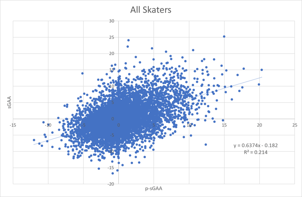
That’s a decent correlation. I have previously done similar calculations for 5v5 on ice xG, and the predictability is pretty much the same. But sGAA correlates much better with goal differential than on ice xG.

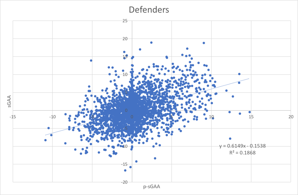
I have also looked at the correlation for forwards and defenders individually. Unsurprisingly, forwards are a bit more predictable:

Adjusting for retired players:

The only adjustment I will make to p-sGAA in this article is due to retired players or players who didn’t make the team. I have deleted the p-sGAA for all of these players, but since most of these players are below average it means that p-sGAA > sGAA. So, I have to adjust for this to make sure the average p-sGAA is 0.

You can do this a few different ways. I have decided to make the adjustment based on projected ice time (p-TOI). So, I have divided the forwards and defenders into groups based on their projected ice time. Within these groups I have adjusted p-sGAA so that it equals sGAA.

Forwards:

p-TOI	No. of players	p-sGAA	sGAA	Difference per player
0	893	0.0	-200.7	-0.225
1-100	860	-138.1	-331.3	-0.225
100-300	830	-372.1	-375.5	-0.004
300-600	797	-582.5	-574.8	0.010
600-900	780	-539.0	-558.7	-0.025
900-1200	935	76.8	-113.1	-0.203
1200+	1207	3444.3	2137.2	-1.083

Defenders:

p-TOI	No. of players	p-sGAA	sGAA	Difference per player
0	458	0.0	-4.1	-0.009
1-100	336	-10.5	-30.9	-0.061
100-300	337	-96.9	-66.0	0.092
300-600	385	-133.9	-168.1	-0.089
600-900	341	-147.5	-142.1	0.016
900-1200	333	-115.6	-53.9	0.185
1200+	1083	1307.5	455.4	-0.787

It doesn’t increase the correlation, but now the overall p-sGAA = sGAA which we want since sGAA correlates directly to goal differential on the team level. It also means that rookies are now expected to perform slightly below average.

Here’s the adjusted correlation:

Projecting team performance:

A big part of the reasoning for making a model like this is to predict how teams will perform in the future. To do so, I need to assign the players to teams, but since I can’t predict who gets traded during the season, I have assigned players to the team where they started the season.

So, I have found the p-sGAA of each team based on the players at the start of the season. This team p-sGAA is then compared with the actual team sGAA:

Like I said earlier – No model is ever going to be perfect. This is a pretty good correlation, actually. The model has some problems with the God awful teams, but it will never expect the skaters on a team to be worth -100 goals, because no team is that bad 3 years in a row.

I have also looked at the sum of all the seasons from 2010/2011 to 2019/2020. Now the correlation is much stronger:

When the sample size is increased the projection model gets it right.

Discussion:

There’s a few things to be aware of when interpreting the p-sGAA model. The model is very conservative when the sample size is small. If a player only has one season in the NHL, the model will always expect him to regress towards league average. That’s just how the model is constructed.

We can use Kaapo Kakko as an example. Before this season the expectation of him would have been league average or slightly below (p-sGAA of -0.225) with the retirement adjustments. That’s how every rookie is expected to perform.

Kakko ended up with an awful statistical season. His sGAA was -12.0, so according to my model he cost NYR 12 goals in their overall goal differential. For next year his projected sGAA will be:

p-sGAA(Kakko) = (51/108) * -12.0 = -5.67

So, the model still expects him to be bad, but he regresses towards average.

Rebuilding teams are another thing to keep an eye on. It seems like the model generally overrates rebuilding teams. This is probably because most such teams have a lot of rookies or inexperienced NHL’ers. The model will think these players are closer to average than they really are. Overall I think the model construction is quite good, but there are some things to be aware of.

From here on out, I will be careful to distinguish between projection and prediction. The model projects a result based on the input I give it, but there’s no interpretation or analysis included.

Before the start of next season, I plan to do a write up on every team. It will include a projection based solely on the model and a prediction based on my own analysis.

Perspective:

This article only discusses the skaters. That’s not because I’ve forgotten about goaltending, but I will save that for the next piece. Goaltending is a lot less predictable, so I will have to do a bit more adjustments.

Once I have a complete model (skaters+goaltenders) I can start comparing to actual results and other models. It will be interesting to compare my model to Dom Luszczyszyn’s model, since the buildup is very similar.

I will make p-sGAA downloadable once the goaltenders are added.

All stats from http://www.evolving-hockey.com