Projecting future results – Goaltender edition

Abstract:

In the last article, I tried to project future performances of the NHL skaters. In this piece I will add goaltender projections, so we can see how the first draft of the projection model performs.

What if all goaltenders were average?

Before we get to the goaltender projections, let’s try to assume every goaltender is league average. This sounds like an awful assumption, but the goaltender variance is so big that it’s actually not the worst idea in the world.

Here’s the correlation between the skater projection (found in the last article) and team goal differential. I’ve assigned players to the team where they started the season, so I’m not using any hindsight. The data is prorated to 82 games:

Clearly, the model correlates with team performance – even with the assumption that all goaltending is average.

My model is build to project goal differential, but since there’s a good correlation between goal differential and standings points, it’s easy to convert goals in to points. The graph below shows points as a function of goal differential from 2010/2011 to 2019/2020. The data is prorated to 82 games:

If we convert our goal projection (p-sGAA) into a point projection, we get the following graph:

It’s quite difficult to evaluate the projection model simply by looking at a correlation graph. I have therefore made a table with the average goal and point difference between the model and the actual result. I have also added Dom Luszczyszyn’s projections for the last 3 seasons.

Season	Goal difference	Point difference	Dom’s model
10/11	24.7	9.0
11/12	27.7	9.0
12/13	28.3	11.5
13/14	25.8	9.4
14/15	27.4	10.5
15/16	18.1	8.3
16/17	27.9	10.6
17/18	28.2	11.6	12.0
18/19	25.4	7.8	8.1
19/20	23.0	7.7	7.2
Overall	25.6	9.5

So, on average the model is off by 25.6 goals and 9.5 points for each team. Interestingly, the model fared better than Dom Luszczyszyn’s model in two of the three seasons even though it’s only based on the skaters.

This indicates that the p-sGAA works really well for skaters, but as we shall see now, goaltending is a lot more complicated.

Adding goaltender projections:

In a perfect world, adding the goaltender projections would make the model much better. Unfortunately, the world isn’t perfect.

Let’s start off by comparing p-sGK and sGK like we did for the skaters in the last article. The goalie projection is based on the 3 previous seasons, and I’m using the same weight as I did for the skaters. I would have expected a flatter weighing to be better, but the best result came with the same weighing. So, p-sGK is calculated with this formula:

p-sGK(Year_x) = (51/108)*sGK(Year_x-1) + (36/108)*sGK(Year_x-2) + (21/108)*sGK(Year_x-3)

Here’s sGK as a function of the calculated p-sGK:

Not exactly a great correlation. Goaltending is very difficult to predict from year to year, which is what the graph shows.

The next thing I want to do, is to make sure the sum of p-sGK for all goalies equal 0, since that’s how sGK is defined. Right now, p-sGK is well above 0, due to retired goaltenders and goaltenders who played before, but didn’t make an NHL team in the projected season. These goaltenders are typically below average, which explains the p-sGK>0.

I’m using the same approach as I did for the skaters, so I’m adjusting based on projected ice time (pTOI). The table below shows the different groups and the average p-sGK and sGK for each group. So, I’m simply adding the difference to each player within the group.

pTOI	No. of players	Age	p-sGK	sGK	Difference per player
0	150	22.8	0.000	-0.247	-0.247
1-300	126	25.0	-0.060	-0.381	-0.321
300-1200	196	26.6	-0.611	-0.112	0.499
1200-2000	153	29.1	-0.299	-1.850	-1.551
2000-3000	175	30.4	0.857	1.201	0.345
3000+	155	30.4	4.995	1.360	-3.635

It’s worth noting that goaltenders with a pTOI>3000 (more than 55 games the 3 previous seasons) decline the most. Maybe, long term fatigue is a thing for goaltenders? We see more and more teams go with an 1A/1B combo.

Anyway, here’s the correlation between p-sGK and sGK with the “retirement” adjustment:

The adjustment does increase correlation, but goaltending is still pretty much unpredictable.

So, what happens if we try to project team performance (G+/-) solely based on our goaltender projections (p-sGK). We assume every skater is league average. This is clearly not a good way project future team results, but it shows us the isolated correlation between team performance and goaltender projection. Here’s the graph:

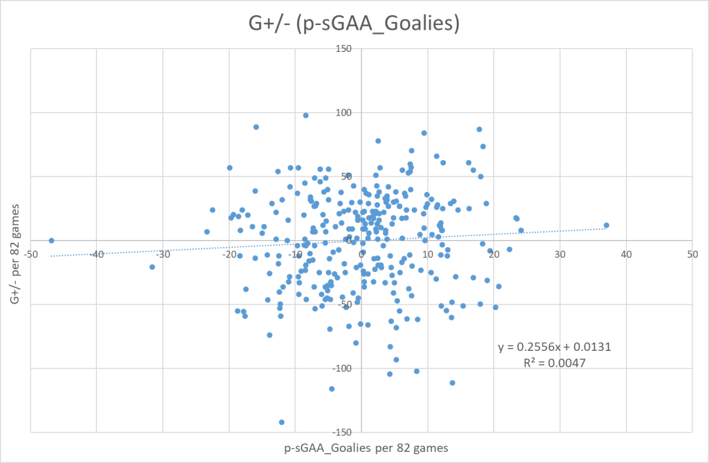
I’m not an expert in statistical modelling, so I don’t know if the following makes sense from a statistical standpoint. I’m using the slope coefficient to determine how much weight to put on the goalie projection. So, the p-sGK is multiplied with 0.2556, meaning the model expects every goaltender to regress 75% towards average.

This will make goaltending seem insignificant in my model, but that’s not because goaltending isn’t important it’s just because I can’t predict goaltending properly. The variance is so big, that I have to weigh the goaltender projections very low.

In the following graph I have calculated p-sGAA like this:

p-sGAA = p-sGAA_Skaters*0.9975 + p-sGAA_Goalies*0.2556 (Using slope coefficients)

Adding goaltenders to my projection makes the model slightly better, but honestly there’s not a huge difference.

We can also project standing points like we did earlier:

And finally we can look at how the model performs from year to year.

Season	Goal difference	Point difference	Dom’s model
10/11	23.9	8.9
11/12	27.7	9.0
12/13	28.2	11.3
13/14	25.1	9.2
14/15	28.1	10.7
15/16	18.1	8.4
16/17	27.6	10.4
17/18	28.6	11.6	12.0
18/19	25.4	7.9	8.1
19/20	22.6	7.5	7.2
Overall	25.5	9.5

Again, adding goaltender projections doesn’t better the model a whole lot.

Adjusting for misses:

How can I improve the goaltender projections then? I’ve tried a lot of different things. One of which was adjusting for misses. On average 72.17% of all unblocked shot attempts hits the net. The xGA a goaltender faces is based on fenwicks against, so a goaltender who faces more shots per fenwick than average is likely to have a lower GSAx.

My assumption here is that the SA/FA ratio will always regress towards league average. One could argue that a good goaltender can force the shooter to miss the net more often than a bad goaltender can. Jonathan Quick does seem to have this ability, but overall I think it’s a decent assumption. Here’s how the adjusted p-sGK is calculated:

p-sGK(miss adj) = p-sGK + (pSA/pFA-0.721664)*pFA*0.09

With this adjustment in place we can see how p-sGK correlates with sGK:

Now, we can go through the same process as earlier. First we find the isolated correlation between team performance and goalie projection:

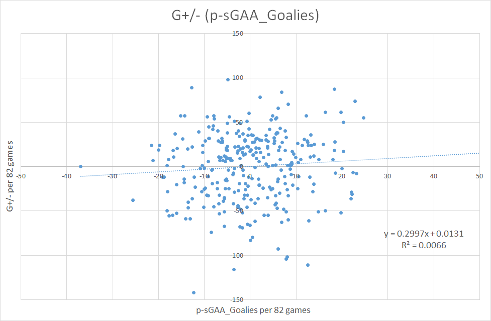
The correlation is better now, which allows me to put more weight on the goaltender projection. The projection is therefore calculated like this:

p-sGAA = p-sGAA_Skaters*0.9975 + p-sGAA_Goalies*0.2997

And that gives us this correlation between team performance and team projection:

Other possible goaltender adjustments:

I have tried to make some other goaltender adjustments to improve the model, but the effects have been minimal. Some of the adjustments work quite well at the individual goaltender level, but doesn’t improve the team projection model.

So, for now I will just leave the model as it is. It makes no sense to add a lot of adjustments that doesn’t really improve the model in the end.

Adding team adjustments:

Instead I will look to some team adjustments. I want to adjust for age and experience. Basically, if a team is young and experienced it’s likely to outperform the model.

So I have found the 20 skaters projected to play the most (highest pTOI) on each team, and looked at their age and experience (pTOI).

The two adjustments are defined like this:

Age_adj: The sum of the 20 players’ age minus the league average that season (the league is getting younger)

Exp_Adj: The sum of the 20 players’ pTOI minus the league average that season.

The new projection can then be found:

p-sGAA = 0.98*p-sGAA_Skaters + 0.2997*p-sGAA_Goalies – Age_adj*0.185 + Exp_adj*0.0036

This gives us the following correlation between goal differential and projected goal differential (p-sGAA):

And here’s the table where we look at the model from year to year:

Season	Goal difference	Point difference	Dom’s model
10/11	21.7	8.3
11/12	27.8	8.7
12/13	28.2	11.2
13/14	23.8	9.1
14/15	26.4	10.5
15/16	19.6	9.1
16/17	26.7	9.8
17/18	29.4	11.7	12.0
18/19	24.0	7.7	8.1
19/20	21.3	6.9	7.2
Overall	24.9	9.3

With the new age and experience adjustments, the model has projected the past 3 seasons better than Dom Luszczyszyn’s model did. It will be interesting to see how the model performs next season and how it compares to Dom’s model.

The complete model can be downloaded in a workbook here.

Discussion:

The goaltending part of the model is still pretty bad, but I think I can make it better. I probably have to combine team projections with goaltender projections. How does team p-sEVD and team p-sSHD affect goaltending? You would expect good team defense to lead to improved goaltending. That’s something worth looking in to.

Overall, I’m quite pleased with the p-sGAA model so far. In the next article I will look at the projections for the 19/20 season in greater detail.

Perspective:

The model as constructed projects full season performances for teams and players. It would be interesting to also project single games in the future.