Talent distribution – Percentiles (part I)

This piece will be the first in a series about talent distribution. I’ve wanted to write about this for a while, but I haven’t really had the time until now. In this article I will focus on skaters and how their “talent” is distributed across percentiles.

What is talent?

The first thing we have to do, is to define talent. Here I’m using my own sGAA model (link), and looking at rates per 60 minutes. I’m also comparing the results to three other models: Evolving-Hockey’s GAR_60 and xGAR_60 (link) as well as TopDownHockey’s GAR_60 (link).

All of these models are descriptive in their nature, so saying they equal talent is perhaps a bit misleading. In reality they try to describe performance rather than talent, but with a big enough sample size talent should equal performance. Plus, talent distribution sounds better than performance distribution.

How is the talent distributed amongst skaters?

Now that we have defined talent, we can look at some distributions. The first thing we look at is talent as a function of percentiles on a seasonal timeframe. In other words, it’s the single season performance of all skaters from 2007 to 2021 as a function of percentiles. I’ve set the minimum TOI requirement to 500 minutes. That gives us close to 8000 players.

So, here’s the sGAA_60 per season as a function of percentile:

There are a few very interesting conclusions to draw from this graph. First of all, we see that talent is not linearly distributed. This isn’t really surprising, but it means that the difference between a 100% player and a 95% player is huge, whereas the difference between a 55% player and a 50% player is relatively small. This is the main reason why ranking players by percentile can be very misleading. In your mind you think a 95% player is close to the best, but that’s not really the truth.

The other important conclusion to draw from the graph is that it is more or less symmetrical. This means that the negative impact per 60 of the worst players is similar to the positive impact per 60 of the very best players. This was somewhat surprising to me.

Finally, my model uses average as the baseline, which is why 50% is close to 0 in sGAA_60. As we shall see below, this is not the case when you use replacement level as the baseline, but more on that later.

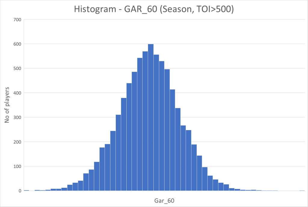
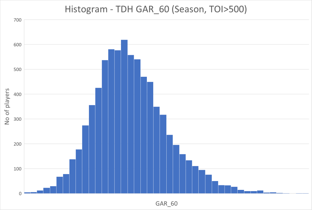
Let’s also take a look at the histogram of sGAA_60. Each column represents a span of sGAA_60 and the height of the column is the number of players within that span.

It looks like a binomial (or normal) distribution. While this is what you would expect based on the percentile graph, I still think it’s somewhat surprising. The concept of replacement level is that you can easily find players at that level, so you would expect many players at this level, and only very few sub replacement level players. This is not what we see though.

I’ve also looked at the histogram of sGAA (totals instead of rates).

Now we multiply by TOI and we see the impact of the bad players decreases, while the impact of the good players increases. This is simply because good players generally play more than bad players.

Comparison to other models

That was the talent distribution according to my model. Now, we will turn our attention towards the distribution of GAR_60/xGAR_60 from Evolving-Hockey and TopDownHockey. Here’s the three models as a function of percentiles.

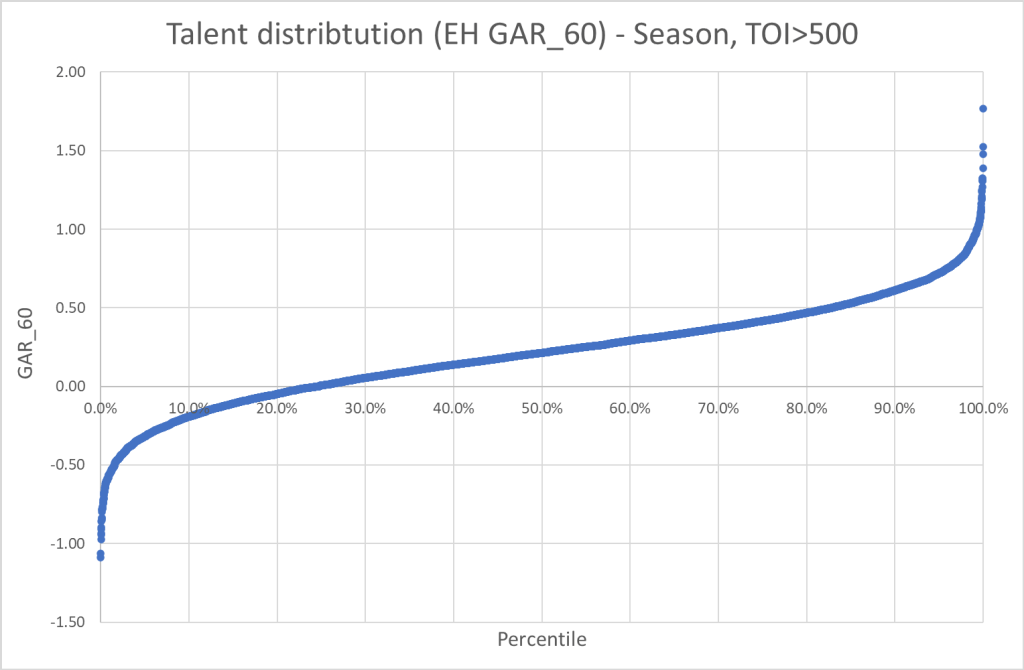
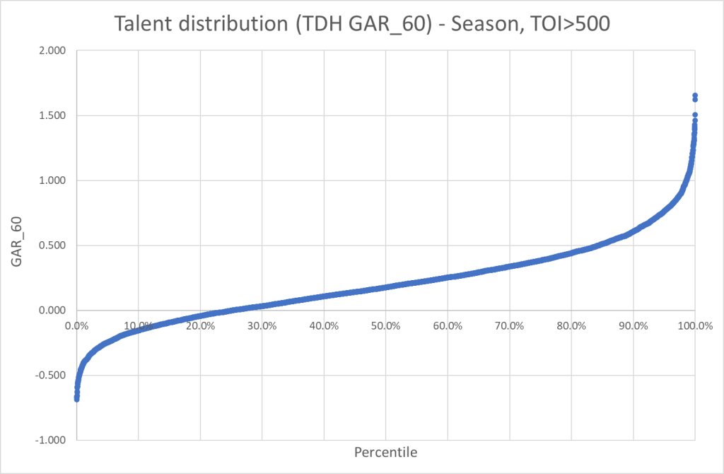
The first thing we see, is that the replacement level is around 25% in all three models, meaning that a quarter of skaters (above 500 minutes) performs at a sub replacement level. Other than that, the graphs look a lot the sGAA_60 one. However, the TopDownHockey model seem to value the impact of good players more than the negative impact of bad players – the graph is not quite symmetrical.

This is also what we see when we look at the histograms.

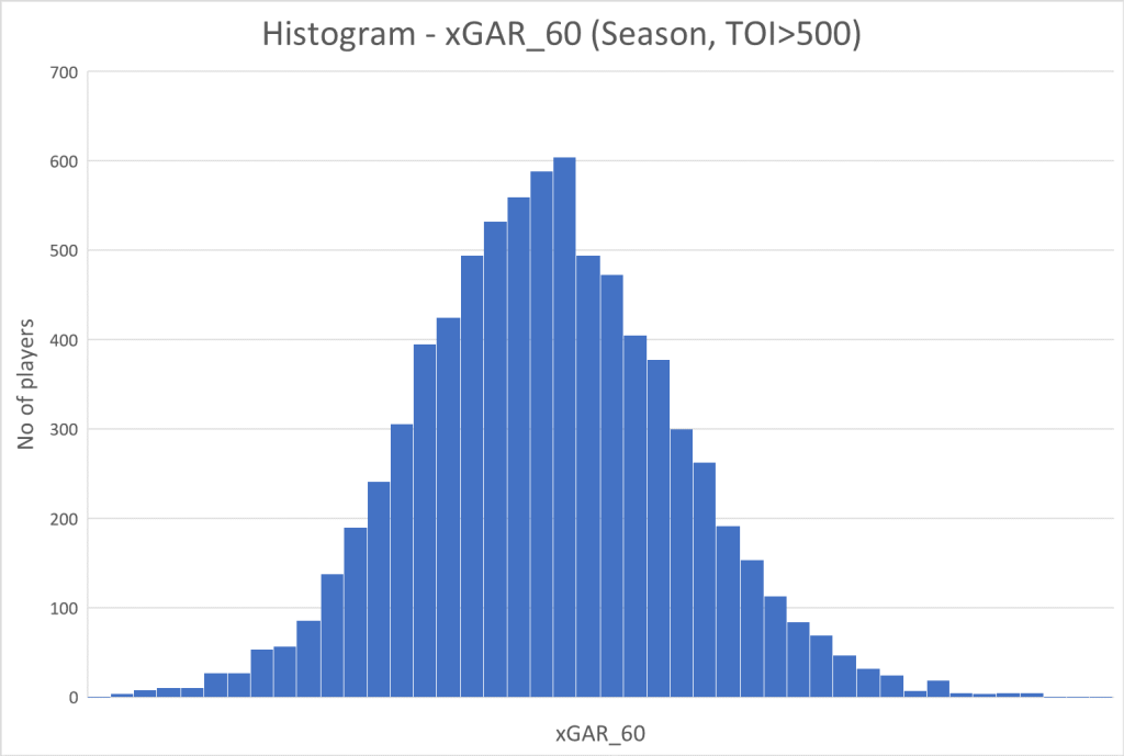
Evolving-Hockey’s models seem to be normally distributed, whereas the TopDownHockey model is skewed slightly towards the better players. I don’t know which is more correct, but it’s certainly an interesting discovery.

Looking at career numbers

So far, I’ve only looked at single season numbers, which might be a flawed approach, since single season data can be heavily influenced by individual and on-ice shooting percentage. Shooting percentage will greatly impact the models, but in the extreme cases it won’t be sustainable.

Therefore, it’s worth looking at career numbers instead. Below are the graphs of the career talent as a function of percentile. The minimum TOI requirement is 4000 minutes, which gives us a dataset of around 850 skaters.

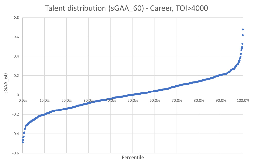
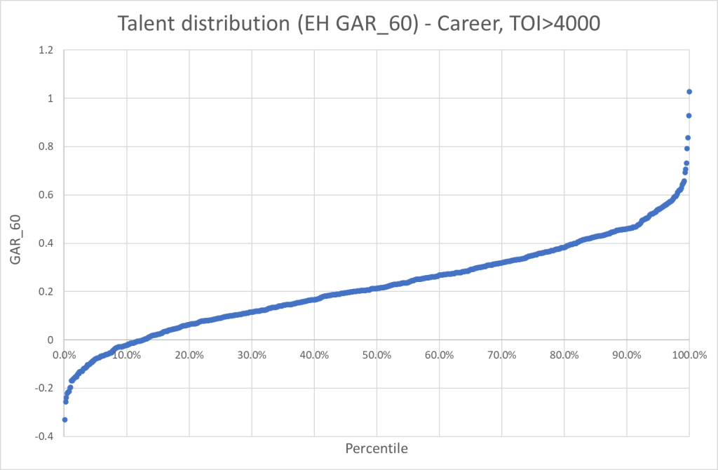
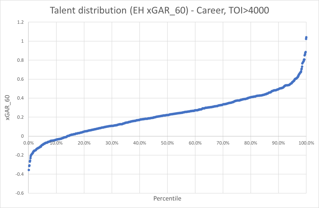
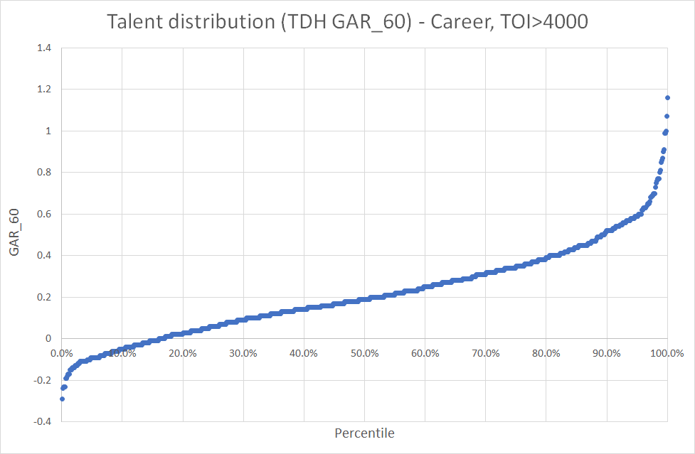
The graphs look similar to the season graphs, but we see fewer sub-replacement level players – between 12% and 17% depending on the model. This makes sense since a lot of sub-replacement level players won’t have long NHL careers (>4000 minutes).

We also see that the scales on the y-axis have changed, meaning the extremities are greater in the single season data. Again, this is fully in line with what we expect.

So just to summarize the career graphs. We still see a small elite tier of players that have very, very impactful careers. We also still see a tier of truly horrendous players, but this group is much small compared to the season data. This is likely because most awful players don’t have long NHL careers, and some players good careers, but are awful towards the end when they get older.

Roster construction perspective

The analysis above opens up for an interesting discussion about roster construction. We clearly see an elite tier of players, but this tier is probably much smaller than most realize. It’s just the top 2-3%. If you can get one these players, you should do whatever it takes to keep him. A Connor McDavid will always outperform his cap hit.

There’s also a tier of awful players well below the replacement level, and surprisingly these players can have a negative impact as great as the one from an elite player. Replacing a player like this, should be the easiest way to improve your team.

If we ignore the top 5% and the bottom 5%, we get the following distribution.

Clearly, the talent in this span is still not distributed linearly, but it’s at least fairly close. In this span it’s all about finding value for money.

Summary: Make sure you replace horrendous players and if you get your hand on an elite player, you do whatever it takes to keep his services. Other than that, it’s all about finding value for money. Make sure you don’t pay elite money for a non-elite player.

In the below graph you can see the talent distribution for every team. Just select the team and season.

Conclusion

• Awful players have similar impact as elite players.
• Sub-replacement level players don’t get replaced (at least not in within the season). You would expect the distribution graphs to flatten around the replacement level, yet we don’t see that.
• The tier of elite players is much smaller than people realize.
• Ranking players by percentile can be very misleading is you’re not aware of the distribution.

Data from Evolving-Hockey.com and TopDownHockey