Talent Distribution – Predictability (Part II)

I didn’t really plan to discuss predictability in this series about talent distribution, since the two are not directly connected. However, I was asked about it, and it does open up for a good discussion about descriptive vs. predictive modelling. I recommend reading part 1 before you read this piece.

Descriptive vs. Predictive models

The names pretty much explain the difference. A descriptive model is built to best describe past results, whereas a predictive model attempts to predict future results. A model can be both descriptive and predictive, but it’s important to understand the difference and the purpose of the model.

When we look at player models, you could say that a descriptive model describes performances and a predictive model estimates future performances based on the current talent level. So, a descriptive model estimates performance and a predictive model estimates talent.

All the models from part 1 are primarily meant to be descriptive models, but today we will look at their predictive power. I think most of these models also have a predictive counterpart, typically called projected WAR or something similar. My predictive model is called p-sGAA, where the p stands for projected. These predictive versions will often include 3 years of weighted data and an age adjustment (there could be other differences as well).

In hockey, goals are the ultimate descriptive metric. The whole purpose of the sport is to outscore your opponent. So, it’s very easy to describe team performance, since the performance is directly equal goal differential or number of standing points. The problem is that goals are not very predictive.

This was why advanced stats like corsi or expected goals were introduced. They are more predictive, more sustainable. The reason for this, is of course that corsi/xG is based on many more events, so the sample size increases much faster. So, corsi predicts corsi much better than goals predict goals, but that in itself is not really interesting. However, it also turns out that corsi/xG predicts future goals better than goals does, and that’s why these stats are relevant.

The difficulty of player evaluation in a team sport

When you evaluate team performance, it’s pretty straight forward. A successful team wins hockey games and outscore their opponent. A bad team can have short term success, because of unsustainable effects. But if a team keeps winning, then they are per definition a good team.

For individual players things are a lot more complicated. We want to isolate the individual players impact, but that’s difficult when there are 11 other players on the ice. GAR models and RAPM models attempt to isolate player impact, but it’s not an exact science, and we can’t easily prove or disprove the correctness of the output.

The only known fact we have, is that the impact of all players on a team should equal the overall team performance. Therefore, I’ve calibrated my model to describe team performance (team G+/-). It’s the only fact we know. This means that team sGAA ≈ team G+/-.

Building the model this way, I know that the sum of all player contributions on a team add up to the actual team result (G+/-), but I still don’t necessarily know that each individual contribution is correct.

Here’s team sGAA as a function of team goal differential:

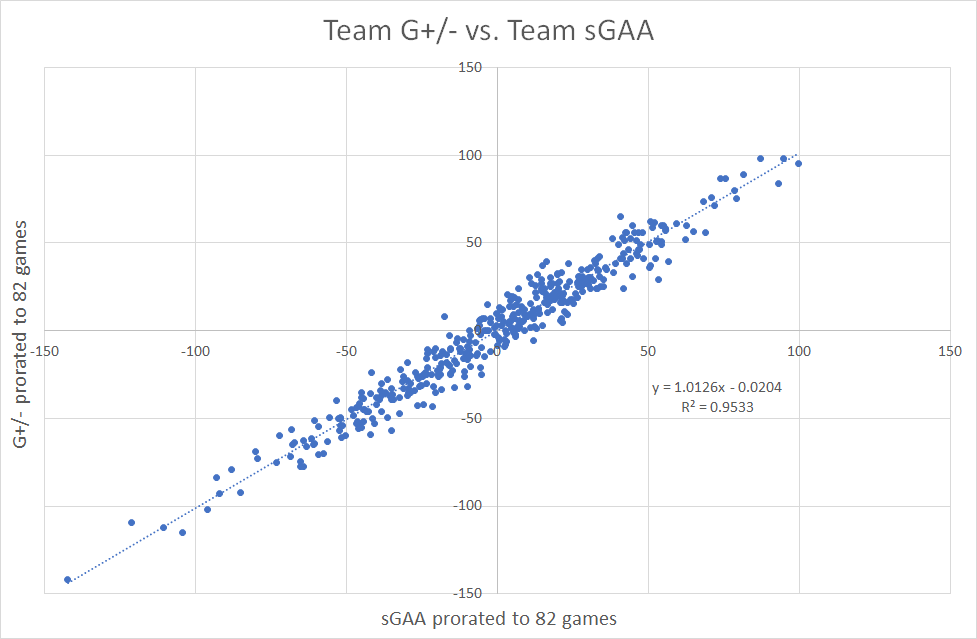
The team sGAA includes skater sGAA and GSAx (goaltending). Considering the great correlation, I’m very confident in the descriptive power of my sGAA model at the team level.

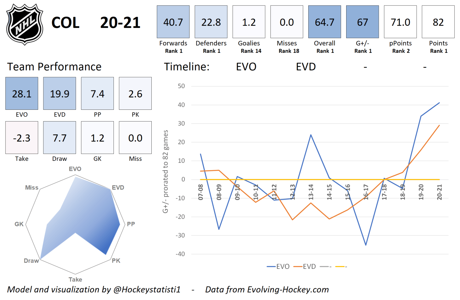
In my team cards you can find the performance of each team from 2007 to 2021, and there’s a short explanatory video here:

That was a fairly long introduction, but the main takeaways are:

• GAR/RAPM models attempt to isolate individual player impact.
• It’s very difficult to prove how well the models succeed in isolating the player impact. We don’t really have anything to hold it up against.
• At the team level the models must correlate well with team goal differential.
• GAR models are generally descriptive, so they describe performance. The predictive counterpart (projected GAR or p-sGAA) attempts to project future performances. In other words, the predictive models are a measurement of talent.
• Go check out the team cards – I think they are pretty cool.

The predictive power of each model

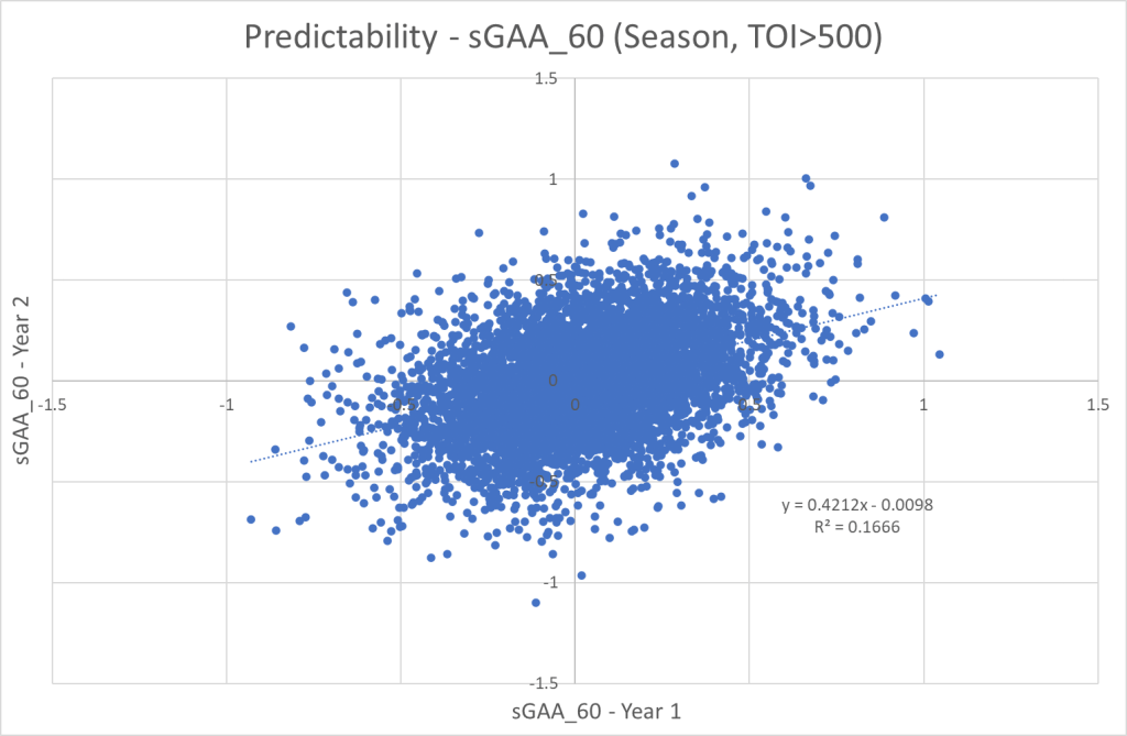
Now we turn our attention to the main focus of this article. How well does past sGAA_60/GAR_60 predict future sGAA_60/GAR_60? To answer this question, I’ve simply looked at the correlation between sGAA_60 in year 1 and sGAA_60 in year 2. To qualify the player must have played minimum 500 minutes in both seasons.

Here are the results from my model, Evolving-Hockey’s models and TopDownHockey’s model.

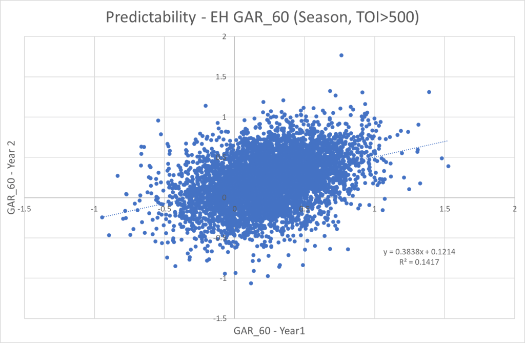
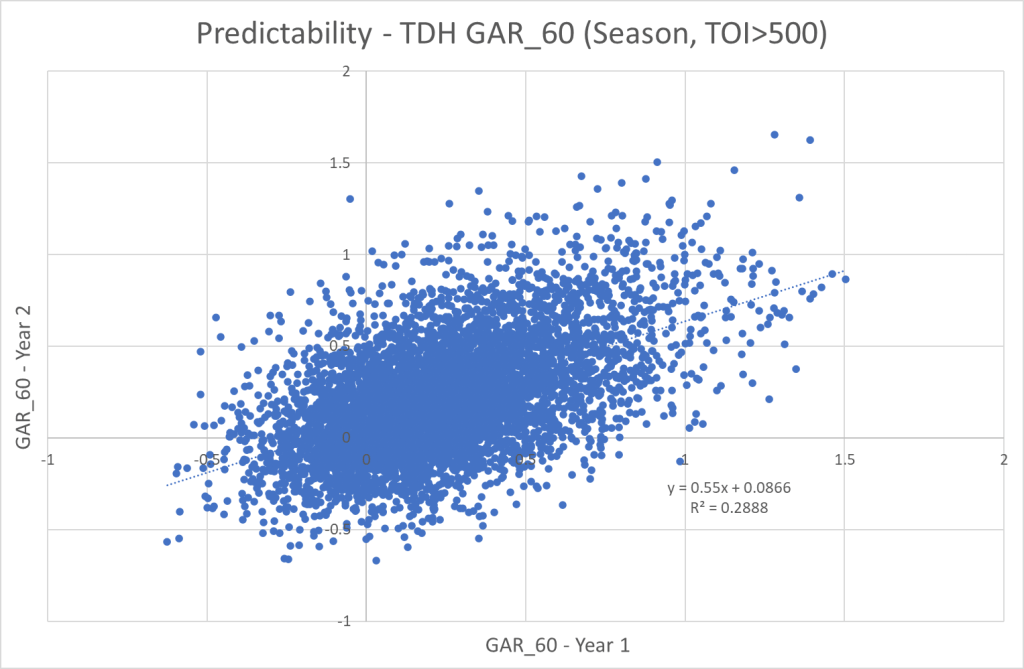
We clearly see that the TopDownHockey model has the best predictive power from season to season. This in itself doesn’t necessarily mean it’s the best model. We have to also consider the descriptive power of each model. The problem is that it’s incredible difficult quantify the descriptive power though.

In reality I don’t really think it’s particularly interesting to know how well GAR predicts GAR. The interesting thing is how well projected GAR predicts actual GAR. We want our predictive model to predict our descriptive model. That’s what we should be testing, but I don’t have that data available at the time. Based on the above results I would still expect the TopDownHockey model perform best in such a setting.

Instead of running more tests, we can discuss why TopDownHockey’s model has a higher predictability than Evolving-Hockey’s GAR model.

To simplify things a lot, you can say that EH’s model is based on isolated goal impact, whereas the TDH model is based on playdriving impact (expected goals) and individual shooting. This means that the TDH model give a lot of credit to shooters, while the EH model give more credit playmakers. It also means that the EH model is heavily affected by on-ice shooting percentage, whereas the TDH model is affected by individual shooting percentage.

On-ice shooting percentage is less sustainable and more reliant on teammates, so when we look at small sample sizes (single season data), we get more outlier results in the EH model. Hence, the smaller predictability.

I think you could argue that TDH’s GAR model (and EH’s xGAR model) overestimates shooters, but underrates playmakers. On the other hand, I would be very careful not to put too much weight on single season data in the EH GAR model. As an example, Jared McCann’s GAR_60 in the 20/21 season is the highest ever recorded.

Player evaluation is difficult in hockey, and there are no easy answers! My sGAA is a combination of EH’s GAR and xGAR models, but I don’t which way is the best.

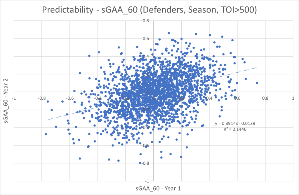
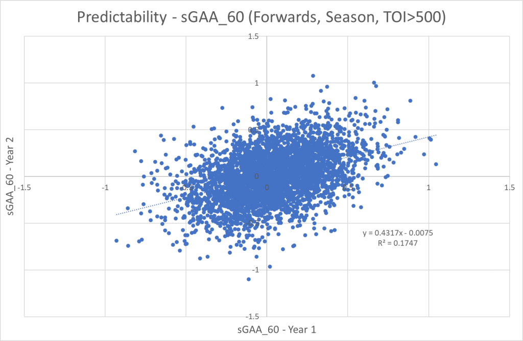
Predictability of forwards vs. defenders

The last graphs in this article show the predictability of defenders and forwards respectively. I’ve only included the graphs from the sGAA model, but all the models show the same trend. Forwards are more predictable than defenders.

Game projection model

I’ve briefly mentioned projected sGAA or p-sGAA, which is my predictive metric. It’s based on 3 years weighted sGAA data, and it’s the primary input in my projection models.

Last season I projected every game, and tracked the results against other models. You can find these results in my model cards and there’s an explanatory video here:

Conclusions

• TopDownHockey has the most predictive model.
• It would be more interesting to research how well projected GAR predicts actual GAR.
• Forwards are more predictable than defenders.
• I promise to discuss talent distribution more directly in the next part of this series.

Data from Evolving-Hockey and TopDownHockey