
In this article I will start building my game projection model. I’d recommend reading the two first articles of the series before you continue reading this post:
The model construction
The idea is to build a game projection model that actually consists of two separate models:
- A pre-season model
- An in-season model
The goal of the pre-season model is to give every player a starting value when the season starts. The goal of the in-season model is to adjust the player values solely based on in-season information.
In the previous articles, I let every player start at the exact same value and then considered how different in-season information would affect the game predictions. In other words, I laid the groundwork for building the in-season model.
For me it’s very important that the in-season model is easily updated. It must be something I can update daily within 5-10 minutes. The preseason model only needs to be updated once every year, so it can theoretically be much more complex.
In this article I will focus on building the in-season model.
Building the in-season model
In the first article, I already looked at the potential variables to include in my in-season model. The next step is to try and combine these variables in the smartest possible way.
There are three parameters I can modify when building the in-season model:
- Which variables to include.
- How many games to gather information from.
- How to weigh recent games vs. older games.
In the previous articles I always used information from the previous 50 in-season games and weighed all the games equally. Theoretically you could use a different number of games and/or weigh games based on recency.
Metric combinations
To a start, I’m just using the data collected in the previous articles. From this data I want to test three different metric combinations:
- EV xG+/-, EV G+/-, PP G+/-, SH G+/-, Individual Points, GSAx
- EV xG+/-, PP G+/-, SH G+/-, GAx, GSAx
- EV xGA, EV GF, PP G+/-, SH G+/-, GSAx
Combination 1 is somewhat similar to Dom Luszczyszyn’s Game Score model, whereas combinations 2 and 3 are similar (although simpler) to Evolving-Hockey’s xGAR and GAR models respectively.
I combined the metrics and refined the data to find the weight of each metric. The results can be found in this table:
| Model | Log loss |
|---|---|
| Combination 1 | 0.6748 |
| Combination 2 | 0.6752 |
| Combination 3 | 0.6759 |
This is the visualization we get, if we look at the log loss as a function of game number. I’ve only included the trendlines to make the graph easier to interpret:
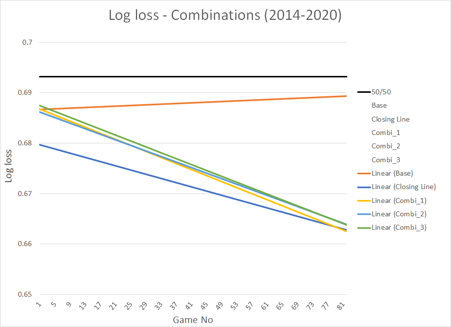
We see that combination 1 is slightly better than combinations 2 and 3. We also see that the log loss of the 3 model combinations is close to the market log loss at the tail end of the seasons.
This is what we get if we zoom in on the last part of the seasons – You could say we give the models 70 games to learn:
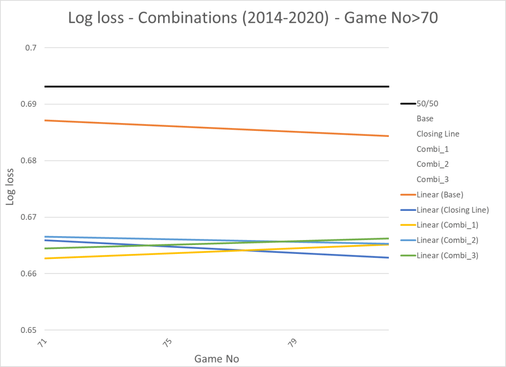
Now the performance of the models is comparable to the market. We also see that the log loss has stabilized, so you could say the models have stopped learning at this point. This isn’t surprising since most players will have played more than 50 games at this point.
Conclusion:
If you combine different variables, you can build a relatively simple in-season model that can compete with the market. The model just needs to be fed enough information.
Combination 1 showed the best results, so this is the combination I will build on. I think you could create a good model based on any of the combinations, but the plan all along was to build a Game Score like metric. So, I’m pleased that combination 1 showed the most promising results.
Number of games to include?
Next step is to try and change the number of games to include in the predictions. So far, I’ve based a player’s value on his performance in the previous 50 in-season games. Changing the number of games to include requires a fair bit of calculations though. For that reason, I’m just changing the number of games to include all in-season games and the last 25 in-season games respectively.
Here’s how changing the number of games affect each variable:
| Variable | Log loss_All | Log loss_50 | Log loss_25 |
|---|---|---|---|
| EV xG+/- | 0.6803 | 0.6794 | 0.6793 |
| EV G+/- | 0.6790 | 0.6790 | 0.6808 |
| PP G+/- | 0.6841 | 0.6840 | 0.6860 |
| SH G+/- | 0.6862 | 0.6861 | 0.6872 |
| GAx | 0.6857 | 0.6854 | 0.6857 |
| GSAx | 0.6862 | 0.6863 | 0.6869 |
| iPoints | 0.6793 | 0.6794 | 0.6809 |
Decreasing the number of games to 25 generally makes the predictions worse. Increasing the number of games mostly has no or limited effect, but it does decrease the predictive power of EV xG+/- quite significantly.
You could of course try to optimize the number of games for each variable, but I think I prefer the simplicity and interpretability of keeping the number of games at 50 for all the variables.
Increasing the weight on recent games
The last thing we can do, is to increase the weight put on recent games. Theoretically, you would like to put more weight on the most recent games. The problem is that it’s difficult to do from a calculation standpoint. The dataset consists of 300K+ rows, and it would require a lot of time and/or computer power to differentiate the weight based on recency (at least with my relatively limited coding/math skills).
I know how to do it, but I’m not sure it’s worth the time and effort required. In the end, you could probably build a slightly better prediction model, but I doubt the difference is worth the effort. I might look in to this later on, but that feels more like an offseason project.
Summary
The in-season model is player-based meaning every player has a value and that value changes based on his performance in the 50 previous in-season games. In building the model I let every player start each season at exact same value (value of 0). This way I can isolate the effect of the in-season model.
I’m going with combination 1, so the model depends on the following variables:
- On-ice EV xG+/-
- On-ice EV G+/-
- On-ice PP G+/- above average
- On-ice SH G+/- above average
- GSAx
- Individual points above average (depending on position and role)
Here’s the prediction performance compared to the market (closing line):
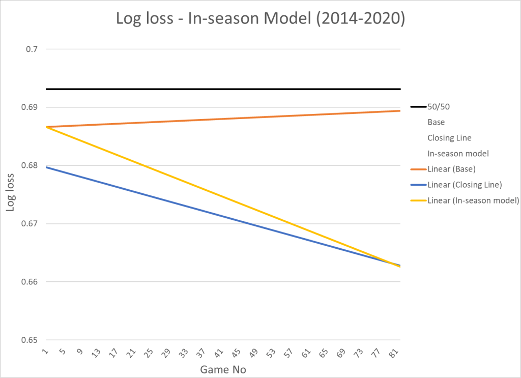
In the beginning of each season the market is obviously doing significantly better than the in-season model – Expecting every player to start the season at the exact same level is not the best approach!
This leads us to the next step: building the pre-season model, so that we can determine a starting value for every player.
From prediction to description
The main goal of the in-season model is to predict the very next game, but what if we used the same model to describe performance.
In other words, what if we calculate a score based on the variables mentioned above and the weight put on each variable will be the same as I used in the in-season model.
Here’s the top 20 seasonal performances (from 14/15 to 19/20) if we do that:
| Player | Season | Score |
|---|---|---|
| CONNOR.MCDAVID | 20162017 | 0.04281 |
| JOE.THORNTON | 20152016 | 0.04239 |
| BRAYDEN.POINT | 20182019 | 0.03967 |
| VICTOR.HEDMAN | 20182019 | 0.03845 |
| CLAUDE.GIROUX | 20172018 | 0.03796 |
| RYAN.SUTER | 20162017 | 0.03767 |
| PATRICE.BERGERON | 20162017 | 0.03713 |
| BRAD.MARCHAND | 20162017 | 0.03694 |
| MARK.GIORDANO | 20182019 | 0.03666 |
| JOE.PAVELSKI | 20152016 | 0.03639 |
| MAX.PACIORETTY | 20192020 | 0.03564 |
| JOHN.KLINGBERG | 20172018 | 0.03406 |
| BRAD.MARCHAND | 20182019 | 0.03404 |
| BRAD.MARCHAND | 20192020 | 0.03362 |
| KEVIN.SHATTENKIRK | 20142015 | 0.03330 |
| MARK.STONE | 20192020 | 0.03320 |
| ALEX.OVECHKIN | 20152016 | 0.03268 |
| RYAN.O’REILLY | 20182019 | 0.03241 |
| JUSTIN.SCHULTZ | 20162017 | 0.03241 |
| PATRICE.BERGERON | 20182019 | 0.03241 |
Perhaps not the perfect top 20 list, but also not the worst list you could come up with. The model isn’t built to be a player evaluation tool, but it does seem to pass the smell test.
These are top 20 best players overall in the entire timeframe:
| Player | Score |
|---|---|
| PATRICE.BERGERON | 0.1610 |
| NIKITA.KUCHEROV | 0.1545 |
| BRAD.MARCHAND | 0.1516 |
| SIDNEY.CROSBY | 0.1496 |
| VICTOR.HEDMAN | 0.1472 |
| PATRIC.HORNQVIST | 0.1344 |
| JOE.PAVELSKI | 0.1338 |
| KRIS.LETANG | 0.1256 |
| RYAN.SUTER | 0.1253 |
| EVGENI.MALKIN | 0.1199 |
| TOREY.KRUG | 0.1183 |
| BRENT.BURNS | 0.1124 |
| DAVID.PASTRNAK | 0.1079 |
| JOHN.KLINGBERG | 0.1049 |
| VLADIMIR.TARASENKO | 0.1039 |
| JARED.SPURGEON | 0.1028 |
| MARK.STONE | 0.1020 |
| STEVEN.STAMKOS | 0.0971 |
| BRAYDEN.POINT | 0.0953 |
| CONNOR.MCDAVID | 0.0943 |
Here’s the top 20 players per 60 minutes (TOI>2000 minutes):
| Player | Score/60 |
|---|---|
| PATRICE.BERGERON | 0.00126 |
| PATRIC.HORNQVIST | 0.00124 |
| BRAD.MARCHAND | 0.00113 |
| NIKITA.KUCHEROV | 0.00113 |
| BRAYDEN.POINT | 0.00108 |
| SIDNEY.CROSBY | 0.00107 |
| ANDREI.SVECHNIKOV | 0.00102 |
| EVGENI.MALKIN | 0.00101 |
| DAVID.PASTRNAK | 0.00100 |
| PAVEL.DATSYUK | 0.00097 |
| JOE.PAVELSKI | 0.00094 |
| ANTHONY.CIRELLI | 0.00092 |
| VICTOR.HEDMAN | 0.00090 |
| VLADIMIR.TARASENKO | 0.00087 |
| JAKE.DEBRUSK | 0.00083 |
| STEVEN.STAMKOS | 0.00082 |
| TOREY.KRUG | 0.00080 |
| KRIS.LETANG | 0.00079 |
| AUSTON.MATTHEWS | 0.00079 |
| CONNOR.MCDAVID | 0.00079 |
Clearly, some players are underrated (Matthews, McDavid, MacKinnon) while others are overrated (Hornqvist)… But the model is relatively simple, so this is to be expected. Even in much more complex player evaluation models (like GAR and xGAR), you’ll find plenty of player rankings you disagree on.
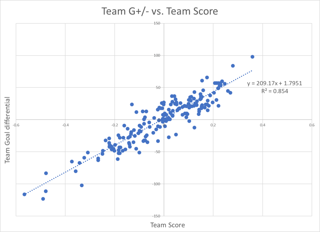
If we sum the player scores for each team and compare it to the team goal differential, we get this correlation:
Perspective
Like I mentioned earlier the next step will be to build the pre-season model and then combine the two models.
My approach to building the pre-season model will be similar to the way I build the in-season model. I will isolate the performance of the pre-season model by not changing the player values as the season progresses.
So, when I built the in-season model I let every player start at the same value and then changed the value based on in-season performance. When I’m building the pre-season model I will find a starting value for each player, and then not change this value throughout the season. This way the two models should be relatively independent when I’m combining them in the end.
Data from http://www.Evolving-Hockey.com

One thought on “Game projection model – In-season Model (Part II)”