Game projection model – The Variables (Part I)

The goal with this series is to build a new game projection model. In this first article I will focus on the different variables/metrics. I want to test how well they predict future results.

The old model

But first a few comments on the old model. It was built on the basis of Evolving-Hockey’s GAR and xGAR models. I started off by creating a descriptive model (sGAA), and then I converted that into a predictive model. This is a decent methodology and it worked well in year one.

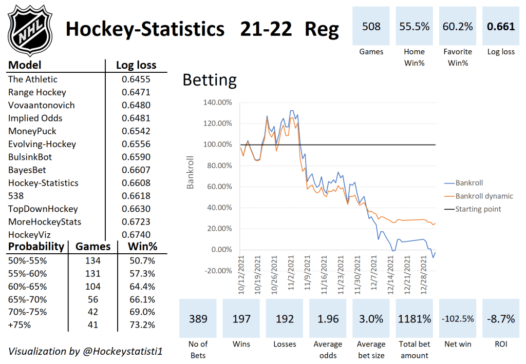
Then this offseason I made some bad model changes. I have likely overfitted the data, and the result is a model that overestimates powerplays and penalties, and underestimates defenders.

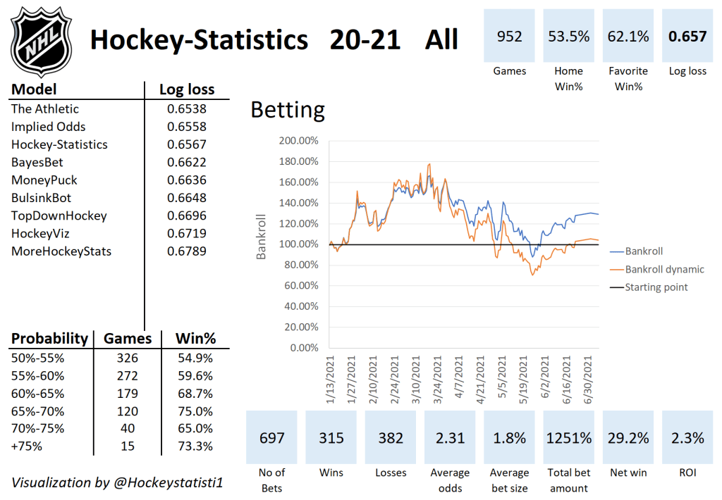
This is how the model has performed this season:

The new model

So, I could just redo the old model, and I would probably end up with a decent model. However, I would rather rethink the entire methodology. Instead of converting a descriptive model into a predictive one, I want to build a predictive model right away. To do this I need to test how predictive the different available variables are – hence this article.

I also want a model that’s easier to update and hopefully easier to interpret.

Preparing the data

I want the model to be player based, so that the game projections depend on the line ups. This complicates things a fair bit, but it should give a better model.

So, before we can start the tests, we need to prepare the data set. The model will be build based on data from 2014/2015 to 2019/2020. I don’t include the 2020/2021 season, because it was shortened, there were no interdivision games and there were no fans in the buildings.

Basically, I want player data on a game basis. I did not include empty net situations, but the data is split into EV, PP and SH columns.

The variables I want to test are:

Even strength on-ice: xGF, xGA, GF, GA, CF, CA

Special teams on-ice: PP G+/-, SH G+/-

Individual stats: G, A1 (primary assists), A2 (Secondary assists), GAx (Goals scored above expected), Penalties taken, Penalties drawn

Goaltender stats: GSAx, GSAx (shot based)

You can find all of these variables in the data file. However, I’m not really interested in simple counting stats. I want to see if a player is better or worse than average (I calculated the averages per second next to the table). Obviously, a forward is expected to score more goals than a defender and on the powerplay you’re expected to score more than you’re at even strength. These things are accounted for by looking at above average stats.

The calculation is simply:

Impact = (Variable_1/second – average/second) * TOI(seconds)

E.g.

xGA impact = (xGA/s – average xGA/s) * EV_TOI

I want to differentiate between forwards and defenders in my testing, so in total this gives us 14 forward variables, 14 defender variables and 2 goaltender variables for testing.

The test set up – Creating baselines

The goal is to see how each variable impact game predictions. To evaluate the impact I’m using log loss, but before we get that far I need to calculate the win probability for each team.

I want to isolate the impact of each variable, so in the beginning I assume all teams are equally strong (the team strength is set at 0.500). This gives us the following win probabilities:

Win prob. = Strength(team)/(Strength(team)+Strength(opponent))

Since the strength of all teams are set at 0.500, the result will always be:

Win prob. = 0.5/(0.5+0.5) = 50%

If the probability is always 50%, then the error of the game predictions will always be 50%, and the log loss will be:

Log loss = -ln(1-error) = -ln(1-0.5) = 0.6931

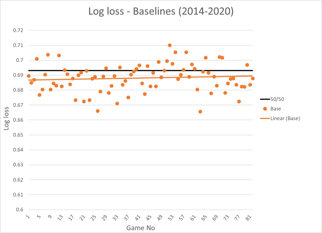
This will be our first baseline. The next step is to adjust for home ice advantage and back-to-back effects. When we do this the win probabilities will be:

Situation	Home	Away
Both teams rested	54.33%	45.67%
Home team B2B	49.78%	50.22%
Away team B2B	58.81%	41.19%
Both teams B2B	54.33%	45.67%

When we calculate the average log loss based on these win probabilities it comes out to 0.6881. This will be our second baseline. If we visualize the log loss as a function of game no, this is the result:

The final baseline I want to create is based on closing betting lines. Now the win probability is calculated based on closing odds (Source: https://www.sportsbookreviewsonline.com/). When we calculate the log loss based on closing lines it comes out to 0.6714 and added to the visualization it looks like this:

In the end we want a model that can compete with the market, so it’s a good baseline to set up. The analysis below will only include the trendlines to ensure that the graphs are easy to interpret.

The test setup – Adding variables

In this test I want to add each variable individually, so I can see how it impacts the log loss. I will still include the home-ice and back-to-back adjustments.

I’m going to let every player start each season at the same level (value of 0), and their value then changes based on their performance above average in the previous 50 in-season games. The team strength is then calculated this way:

Team Strength = 0.500 + SUM(Variable changes)*x

So, the team strength is calculated based on how the line up has performed (in the tested variable) previously in the season. The team strength will therefore always start at 0.500 and then change based on performance in the tested metric/variable.

The x-value is defined as the value where the overall log loss is at its lowest. This way we can test how each variable impact the log loss.

Even strength expected goals

Let’s start by testing the expected goals variables. For defender xGA the lowest log loss (0.6834) was found when x was -0.00654. The x-value is of course negative because having a low on-ice xGA is a good thing.

I did the same thing for forward xGA, defender xGF and forward xGF. You can see the log loss and x-value in the table below.

Variable	Log loss	x	y
Base	0.6881
Closing Line	0.6714
Defender xGA	0.6834	-0.00654
Forward xGA	0.6828	-0.00439
Defender xGF	0.6824	0.00736
Forward xGF	0.6820	0.00485
Combined xG	0.6794		0.372

Finally, I combined all the xG-variables by keeping the x-values constant and then finding the y-value with the lowest log loss:

Team strength = 0.500 + ([D xGA]*-0.00654+[F xGA]*-0.00439+[D xGF]*0.00736+[F xGF]*0.00485)*y

The y-value is below 1, because the variables are dependent. [D xGA] is closely connected to [F xGA] and [D xGF] is closely connected to [F xGF].

In the graph below you see how the log loss changes as the seasons progress. I’m just showing the trendlines to make the graph easier to overview.

There are two things worth noting. xGF appear to be a better predictor of future results than xGA, and [F xG] predicts results better than [D xG]. Perhaps just because there are more forwards on the ice at even strength.

Even strength goals

Next, we will look at on-ice even strength goals. The procedure is the same as for xG, and you can see the results here:

Variable	Log loss	x	y
Base	0.6881
Closing Line	0.6714
Defender GA	0.6842	-0.00385
Forward GA	0.6843	-0.00248
Defender GF	0.6823	0.00444
Forward GF	0.6819	0.00294
Combined G	0.6790		0.448

And here’s the visualization of the trendlines:

Again, we see that GF is a better predictor than GA, but more surprisingly on-ice goals appear to predict results better than on-ice expected goals. This is different from what we see when we simply look at team stats.

Even strength corsi

Here’s the results when we add the corsi variables:

Variable	Log loss	x	y
Base	0.6881
Closing Line	0.6714
Defender CA	0.6838	-0.000331
Forward CA	0.6834	-0.00023
Defender CF	0.6832	0.000323
Forward CF	0.6830	0.000217
Combined Corsi	0.6812		0.337

And here’s the visualization:

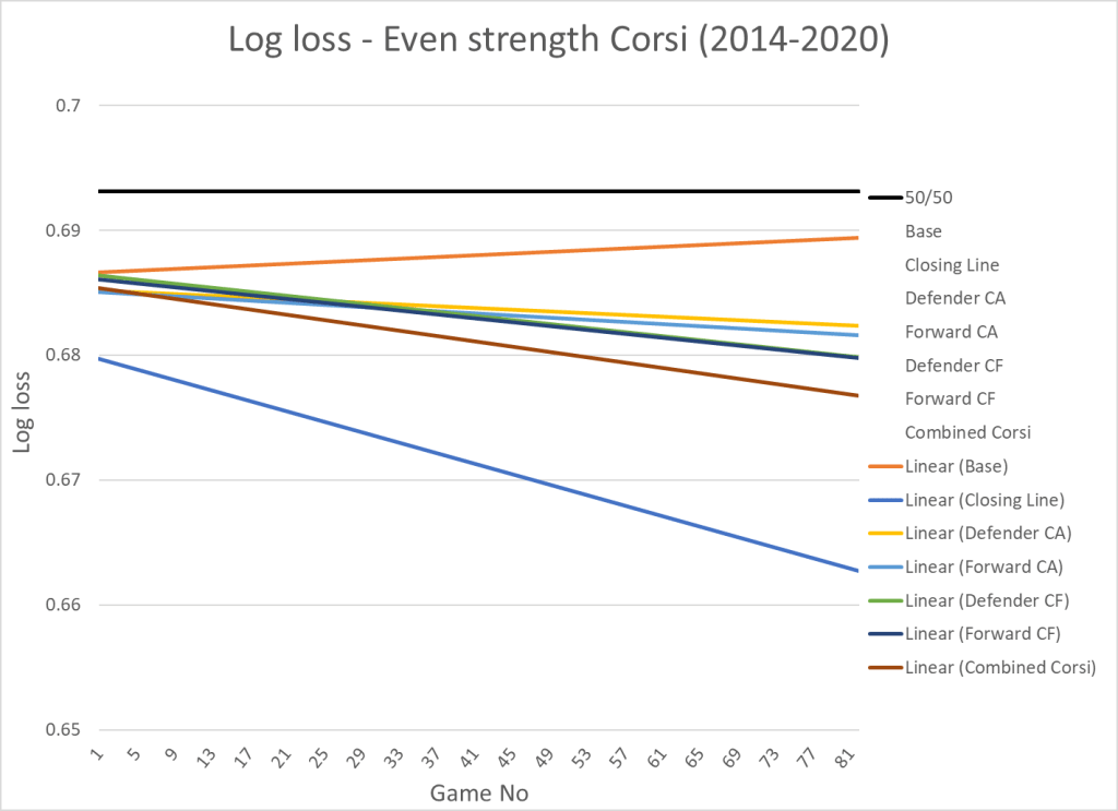
Corsi in this test is a worse predictor than both expected goals and actual goals.

Special teams

The metrics I use for special teams are on-ice PP G+/- above average and on-ice SH G+/- above average. I could have used xG+/- instead, but for special teams I think it’s better to look at the actual results.

Here’s the results of the test:

Variable	Log loss	x	y
Base	0.6881
Closing Line	0.6714
Defender PP	0.6854	0.00833
Forward PP	0.6839	0.00361
Combined PP	0.6842		0.568
Defender SH	0.6862	0.00498
Forward SH	0.6862	0.00498
Combined SH	0.6861		0.531

And here’s the visualization:

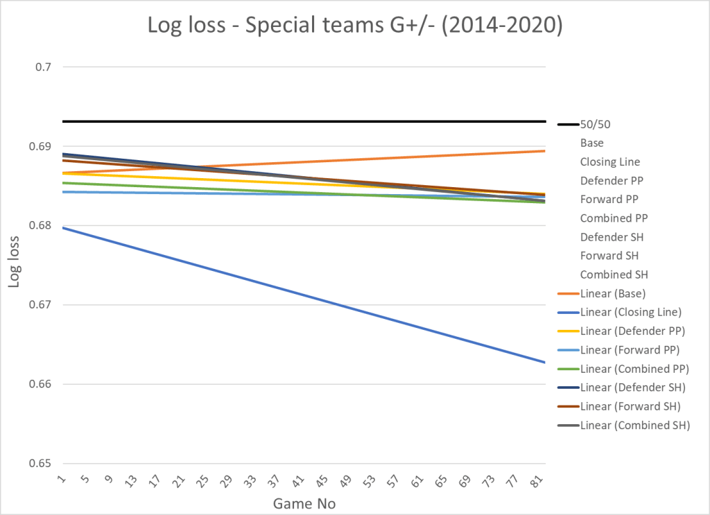
Obviously, even strength performance is more important than special teams performance since most of the game is played at even strength… But accounting for special teams will still improve your model. PP performance appear to be a slightly better predictor than PK performance.

Individual points

When I’m looking at points, I’m using points above average, so I account for position (F or D) and role (EV_TOI, PP_TOI and SH_TOI). Here’s the results:

Variable	Log loss	x	y
Base	0.6881
Closing Line	0.6714
Defender iG	0.6858	0.0132
Forward iG	0.6817	0.00749
Defender A1	0.6852	0.00963
Forward A1	0.6828	0.00771
Defender A2	0.6859	0.00918
Forward A2	0.6825	0.0102
Combined Points	0.6794		0.348

And here’s the visualization:

Individual points seem to be a really strong predictor of future results – especially for forwards. This is probably something that’s underrated by a lot of analytics people, and likely one the reasons why Dom Luszczyszyn’s model is so successful.  

Goals scored above expected (GAx)

I also tested goals scored above expected (shooting): GAx = iG-ixG

Variable	Log loss	x	y
Base	0.6881
Closing Line	0.6714
Defender GAx	0.6878	0.00573
Forward GAx	0.6858	0.00516
Combined GAx	0.6854		0.979

Here’s the visualization:

Defender GAx doesn’t appear to predict future results at all. Forward GAx is a decent predictor. I think there’s too much variance on long range point shots.

Goals saved above expected (GSAx)

I tested two goaltender metrics – normal fenwick based GSAx and shot based GSAx. I don’t think goaltenders have much impact shot misses, so I only want to credit goaltenders with the actual saves. I wrote this article about the subject here.

Variable	Log loss	x
Base	0.6881
Closing Line	0.6714
GSAx (fenwick)	0.6864	0.00605
GSAx (shot)	0.6863	0.00622

Here’s the visualization:

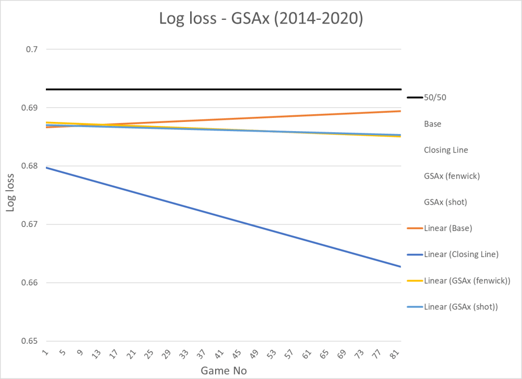
In terms of predictiveness there’s no real difference between the two models.

Penalties

Finally, I tested penalties. Here’s the result:

Variable	Log loss	x	y
Base	0.6881
Closing Line	0.6714
Defender Take	0.6880	-0.00041
Forward Take	0.6877	0.000595
Defender Draw	0.6880	0.00045
Forward Draw	0.6878	0.0006
Combined PEN	0.6875		0.747

And the visualization:

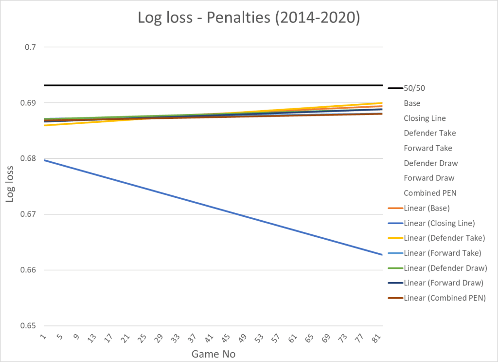
Penalty metrics have little to no predictive value. Adding penalty metrics for forwards might improve your model a tiny bit.

Comparing the variables

That was a lot of tables and graphs, but here’s all the variables sorted from best predictor (lowest log loss) to worst predictor (highest log loss):

Variable	Log loss	x
Forward iG	0.6817	0.00749
Forward GF	0.6819	0.00294
Forward xGF	0.6820	0.00485
Defender GF	0.6823	0.00444
Defender xGF	0.6824	0.00736
Forward A2	0.6825	0.0102
Forward A1	0.6828	0.00771
Forward xGA	0.6828	-0.00439
Forward CF	0.6830	0.000217
Defender CF	0.6832	0.000323
Defender xGA	0.6834	-0.00654
Forward CA	0.6834	-0.00023
Defender CA	0.6838	-0.00033
Forward PP	0.6839	0.00361
Defender GA	0.6842	-0.00385
Forward GA	0.6843	-0.00248
Defender A1	0.6852	0.00963
Defender PP	0.6854	0.00833
Forward GAx	0.6858	0.00516
Defender iG	0.6858	0.0132
Defender A2	0.6859	0.00918
Forward SH	0.6862	0.00498
Defender SH	0.6862	0.00498
GSAx (shot)	0.6863	0.00622
GSAx (fenwick)	0.6864	0.00605
Forward Take	0.6877	0.000595
Defender GAx	0.6878	0.00573
Forward Draw	0.6878	0.0006
Defender Take	0.6880	-0.00041
Defender Draw	0.6880	0.00045

The best predictors are individual forward points and offensive on-ice stats (GF and xGF). This is definitely something to keep in mind, when we get around to actually building the model.

Perspective

The next step will be to combine the best variables in a smart way. Most of them are dependent on each other, so we can’t just include all of them… But that will be the subject for the next article in the series.

Data from www.Evolving-Hockey.com and www.sportsbookreviewsonline.com