
In this article I will take a first crack at building an xG model from scratch. As with most things I do, the approach is slightly different from the other public xG models.
Background and purpose:
Before we get to the actual model building, it’s important to understand what an xG model is… And what we want it to be.
This is my definition of xG taken from my book: Introduction to Advanced Hockey Statistics.

So, we want the xG model to estimate the value of each shot. However, xG value and goal probability aren’t necessarily the same thing. I want my model to estimate the shot value with average goaltending and average shooting. A slap shot by Alex Ovechkin clearly has a higher probability of going in, than a slap shot under the same conditions by Joe Thornton… But we still want the xG values to be the same, so that can we use xG to evaluate the quality of shooters and goaltenders.
You can say that an xG model has two purposes: Describe past results (descriptive model) and predict future results (predictive model).
xG as a descriptive model:
We’ve already discussed the descriptive nature of an xG model. It estimates the shot value, which allows us to determine how much shot value we created (xGF) and how much shot value we allowed (xGA). But we can also determine how much better than average the shooting was (GAx = GF – xGF) and how much better than average the goaltending was (GSAx = xGA – GA).
Here’s a shot hierarchy showing the relationship between the different shot metrics:

Expected goals is a way to include shot quality in your analysis… instead of just counting shots (quantity).
It’s very important that we can use the xG model to differentiate between play driving (xGF%) and goaltending/shooting. That’s why I don’t want to include shooter or goaltender information in my xG model.
The goal is to describe shot value for an average shooter against an average goaltender. The goal isn’t to describe goal probability!
xG as a predictive model:
The other important feature of expected goals is to predict future results. It turns out that play driving (xGF%) is a pretty good predictor of future results (GF%). This makes xG an important component in projection models. If the goal is to predict season results, then it’s important to have a great predictive xG model.
In other words, we want our xG model to be both a good descriptive model and a good predictive model.
Evaluating xG models:
You typically measure xG model performance with log loss and AUC. Without going into details, these metrics measure the model’s ability to describe goal probability on each shot. However, this isn’t exactly what we want the xG model to be. First of all, log loss and AUC only measure the descriptive value of the model, not the predictive value. Secondly, they measure goal probability rather than shot value by an average shooter against an average goaltender.
Anyway, log loss and AUC are still decent evaluation tools, but they won’t tell the whole truth. Nonetheless, they should give us an indication of model performance.
Ideally, we would like to also test the predictive value of the xG model!
Just to summarize real quickly:
- We want to use the xG model to describe results: Shooting, Shot Generation, Shot Prevention, Goaltending -> Player Evaluations, Team Evaluations. (it’s important that the model can distinguish between shooting/goaltending and play driving).
- We want to use the xG model to predict future results -> Season Projections, Game Projections, Player Projections.
- Log loss and AUC aren’t perfect measures for xG models… but they are still good indicators of model performance.
Creating a baseline:
My approach is to build a baseline model based on 5v5 shot location and then simply adjust this baseline model based on other parameters.
Here’s how I created the baseline:
- Scraped all Play-By-Play data from 2007 to 2022 (both regular season and playoffs) using Harry Shomer’s PBP scraper.
- Removed all shot attempts that doesn’t have a shot location (mostly shots from the early seasons).
- Divided the ice into small boxes.
- Counted 5v5 unblocked shot attempts (fenwick) and goals in each box.
- Calculated 5v5 FSh% in each box (FSh% = Goal/Fenwick). This is my xG_base!
The image below shows the FSh% of all the boxes:
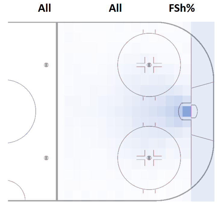
You can find the xG values for each box in this document.
The idea is to use this very simple model as the base of the xG model. Everything else is just adjusting the base model based on different parameters.
The log loss of xG_base is 0.1967 (5v5) and 0.2192 (All strengths – without empty net situations). Considering how simple the model is, these results are actually surprisingly good. This just goes to show that shot location is the most important variable in any public xG model.
I’ve decided to categorize shots in 6 strength states:
- 5v5
- 4v4
- 3v3
- PPv4 (5v4)
- PPv3 (5v3 or 4v3)
- SH
I’ve elected not to include empty net situations and penalty shots to the xG model. I might add in game penalty shots later on, but I don’t want to include empty net situations. I think they can really skew the data, so I think it’s preferable to ignore xG in those situations.
Next step is to add the adjustments.
I’m going to build 6 separate models – One for each strength state. We will start off by building the 5v5 model.
Building the 5v5 model:
In the first version of this xG model I will adjust based on the following parameters:
- Rebound shot (Shot taken within 2 seconds of the previous shot is defined as a rebound shot)
- Rush shot (Shot taken within 4 seconds of an event from the neutral or defensive zone)
- Shot type (e.g., Slap shot, wrist shot, etc.)
- Score state (e.g., trailing by 2, leading by 1, tied, etc.)
- Rink Bias (Differences from arena to arena)
- Season (Differences from season to season, for example due to smaller goalie equipment)
You could definitely add more adjustments, but in this pilot version of the xG model I will keep it simple.
The idea is to simply multiply the adjustments to the xG_base model:
xG = (xG_base)*(Rebound adj.)*(Rush adj.)*(Shot type adj.)*(Score state adj.)*(Rink Bias adj.)*(Season adj.)
Running the first adjustments:
We will start off by adding adjustments for rebounds, rushes, shot type and score state. We will do it in 3 steps:
- Rebounds and rushes
- Shot type
- Score state
We simply adjust based on Goals per xG_base. So, we look at all 5v5 rebound shots and calculate: Goals(rebounds) per xG_base(rebounds). This value is around 2, so a rebound shot is two times more likely to go in, than a non-rebound shot from the same location.
Then we do the same thing for rush shots (around 1.7), and after that we re-calculate the xG:
xG(1) = (xG_base)*(Rebound adj.1)*(Rush adj.1)
Next step is to add adjustments for shot type, so we simply find Goals per xG(1) for each shot type: Slap shot, wrist shot, backhand, tip-in, snap shot, wrap-around and deflection.
xG(2) = (xG_base)*(Rebound adj.1)*(Rush adj.1)*(Shot type adj.1)
Then you do the same thing based on score state:
xG(3) = (xG_base)*(Rebound adj.1)*(Rush adj.1)*(Shot type adj.1)*(Score state adj.1)
That’s one cycle. Then we re-run the cycle until the adjustments remain the same. It took 6 cycles for the adjustments to stabilize.
Rink Bias:
Next step is to adjust for rink bias. There is no perfect way to do this since the problem is that the data itself is flawed.
My estimation is that the shot quality (xG per fenwick) at home should be equal to the shot quality away. Obviously, some teams may play a different style at home vs. away, but I still think the shot quality should be relatively stable, home vs. away. The total xG might differ a fair bit, but this is why I’m using xG/F instead of total xG.
Anyway, I’m just adjusting for rink bias this way:
Rink Bias adj. = (Shot Quality away)/(Shot Quality home)
Again, I ran a few cycles until Rink Bias adj. remained the same. You can find the rink bias adjustments here.
If the value is below 1, it means that shots generally are tracked too close to the net (e.g., NYR, NYI, EDM). If the value is above 1, it means that shots generally are tracked too far away from the net (e.g., MIN, T.B, BOS, BUF).
I’m using 5v5 data to calculate the rink bias, so the rink bias adj. will remain the same for all the other strength states as well. If shots are tracked too close to the net at 5v5, the assumption is that it’s also the case at the other strength states.
Season adjustment:
The final adjustment is based on season. I want the total xG to equal the total goals for every season. You can argue for and against that (other xG models don’t do this).
This means that the total GSAx and GAx in a season always adds up to 0. In other words, we’re always comparing performance to the other players in the same season.
The final 5v5 model:
After I added the season adjustments, I ran all the adjustments one more time, to ensure they were still stable.
Here’s all the 5v5 adjustments:
| Adjustment | Specification | Value | Strength state |
|---|---|---|---|
| Rebound | 2.130 | 5v5 | |
| Rush | 1.671 | 5v5 | |
| Shot type | Wrist | 0.865 | 5v5 |
| Shot type | Slap | 1.168 | 5v5 |
| Shot type | Backhand | 0.657 | 5v5 |
| Shot type | Tip-In | 0.697 | 5v5 |
| Shot type | Snap | 1.137 | 5v5 |
| Shot type | Wrap-around | 0.356 | 5v5 |
| Shot type | Deflected | 0.683 | 5v5 |
| Score state | -3 or less | 0.953 | 5v5 |
| Score state | -2 | 0.991 | 5v5 |
| Score state | -1 | 0.980 | 5v5 |
| Score state | 0 | 0.971 | 5v5 |
| Score state | +1 | 1.031 | 5v5 |
| Score state | +2 | 1.109 | 5v5 |
| Score state | +3 or more | 1.107 | 5v5 |
The 5v5 log loss is now down to 0.1925 and the AUC is 0.7720.
Building models for the other strength states:
I did the exact same thing for all the other strength states, and you can find all the xG adjustments in this document.
I didn’t adjust all the strength states based score state, because the sample size was limited. For instance, we don’t have a lot of data from 3v3 hockey, when the teams aren’t tied considering almost all the 3v3 data comes from overtime.
Evaluating the model:
Testing descriptive value:
We’ve already discussed some of the limitations with using log loss and AUC for xG model evaluations, but they are still useful. Here’s the log and AUC for each strength state and all strengths (minus empty net situations):
| Strength state | Log loss | AUC |
|---|---|---|
| All Strengths | 0.2098 | 0.7634 |
| 5v5 | 0.1925 | 0.7720 |
| 4v4 | 0.2137 | 0.7500 |
| 3v3 | 0.3466 | 0.6662 |
| PPv4 | 0.2833 | 0.6968 |
| PPv3 | 0.3937 | 0.6506 |
| SH | 0.2099 | 0.8133 |
We could also look at the log loss and AUC season for season:
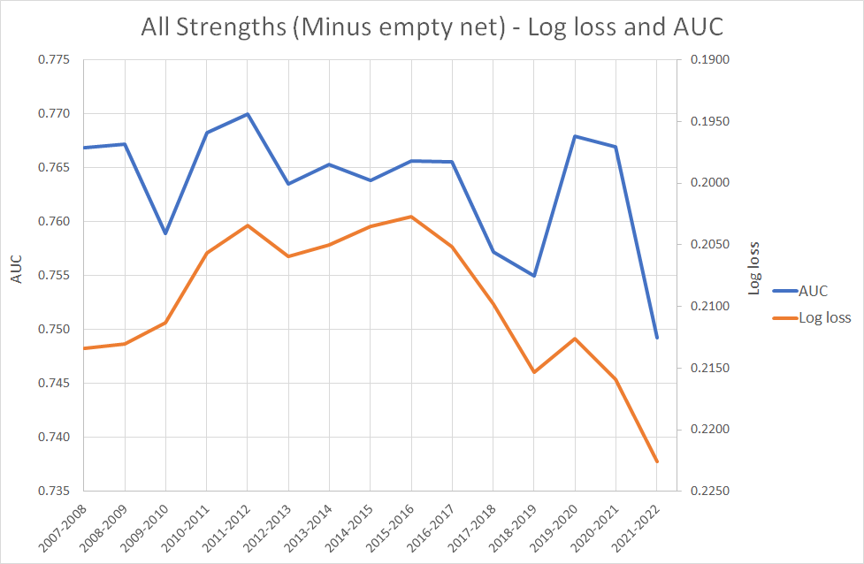
We see a trend where especially the log loss is getting worse and worse. This is probably not because the model is doing worse in the later seasons. It’s likely because teams are taking less low danger shots and more high danger shots. These are more difficult to predict and will therefore have a higher (worse) log loss.
If we compare log loss to the average shot value (xG/F), we clearly see that the two are connected:

Other xG models:
From what I can find most other public models are around 0.77 AUC and 0.20 log loss. So, in terms of descriptive performance my model isn’t better than the other public models, but it is competitive.
I think this is a good starting point, considering there are quite a few other parameters we can add to the model.
Most other models are built via gradient boost, and that may still be the best approach, but this way of model building appear to be competitive which is exciting. In the end, the models are probably very similar. We just got there in different ways.
Testing predictive value:
I would like to do a more comprehensive test of the predictive value, bur for now this will do. In my book, I tested how well a team’s xGF% (Evoving-Hockey’s xG model) in the first 41 games of a season correlated with GF% (result) in the last 41 games of the season. In other words, I tested how well the xG model could predict results of the second half of a season.
Here’s the results:

The R^2 value was 0.4859. I did the exact same test with my xG model and results were pretty much the same (R^2 = 0.4852).
GSAx:
The final model test is more of the anecdotal kind. Here’s the top goaltenders in terms GSAx (both regular season and playoffs):
| Goaltender | GSAx |
|---|---|
| HENRIK LUNDQVIST | 138.9 |
| TUUKKA RASK | 114.9 |
| CAREY PRICE | 101.8 |
| JAROSLAV HALAK | 98.8 |
| SEMYON VARLAMOV | 96.6 |
| CORY SCHNEIDER | 93.4 |
| JONAS HILLER | 88.8 |
| ANDREI VASILEVSKIY | 88.8 |
| TOMAS VOKOUN | 85.9 |
| JONATHAN QUICK | 84.4 |
| FREDERIK ANDERSEN | 82.6 |
| BRADEN HOLTBY | 80.3 |
| CONNOR HELLEBUYCK | 78.9 |
| IGOR SHESTERKIN | 78.0 |
| RYAN MILLER | 77.0 |
| JUUSE SAROS | 72.9 |
| MARC-ANDRE FLEURY | 72.0 |
| BEN BISHOP | 71.4 |
| ROBERTO LUONGO | 68.9 |
| JOHN GIBSON | 67.6 |
This seems like a decent list. At least there’s nothing too crazy here. Roberto Luongo is probably lower than you would expect. Igor Shesterkin just had the best season recorded (since 2007), so he’s very high already.
Perspectives:
There are a few additions I would like to make to the model.
- Make rebound adjustment dependent on time since last shot – A rebound in the same second as the previous shot is worth more than a rebound after 2 seconds.
- Factor in angle change and time since last event – It affects the goaltender’s pre-shot movement and reaction time.
- Position of the shooter (as in forward or defender) – I think forward shots are more dangerous than defender shots.
I may want to add a few more things, but this is what I can come with right now.
Eventually, I would also like to build a shot-based xG model. When it comes to goaltender evaluations, I think it’s better to judge them based on shots faced rather than fenwicks faced. I don’t think goaltenders have that much influence on shot misses.
The goal is to use a shot based xG model to find GSAx. I would still use the fenwick based xG model for everything else.

One thought on “Building an xG model – v. 1.0”