Introduction To Hockey Statistics – First Chapter

You can find the full book here: https://hockeyskytte.gumroad.com/l/Hockey-Statistics

Table of contents

1. Introduction
2. Shot Statistics
   2.1 Shot Hierarchy
   2.2 Shot Formulas
   2.3 Shot Tracking
   2.4 Summary
3. Predictability
   3.1 Descriptive vs. Predictive
   3.2 Test setup
   3.3 Results
   3.4 Conclusion
   3.5 Sustainability vs. Luck
   3.6 Summary
4. Data categories
   4.1 Team-, Individual- and On-Ice Statistics
   4.2 Macro Stats vs. Micro Stats
   4.3 Player models
5. Analyzing a team sport
   5.1 Productivity
   5.2 Output vs. talent
   5.3 Summary
6. Data Interpretation
   6.1 Biases
   6.2 Sample size
   6.3 Context
   6.4 Knowledge and Creativity
7. Data Sources
   7.1 Statistics sources
   7.2 Play-By-Play data
   7.3 Summary
8. Hockey-Statistics.com
9. Conclusion

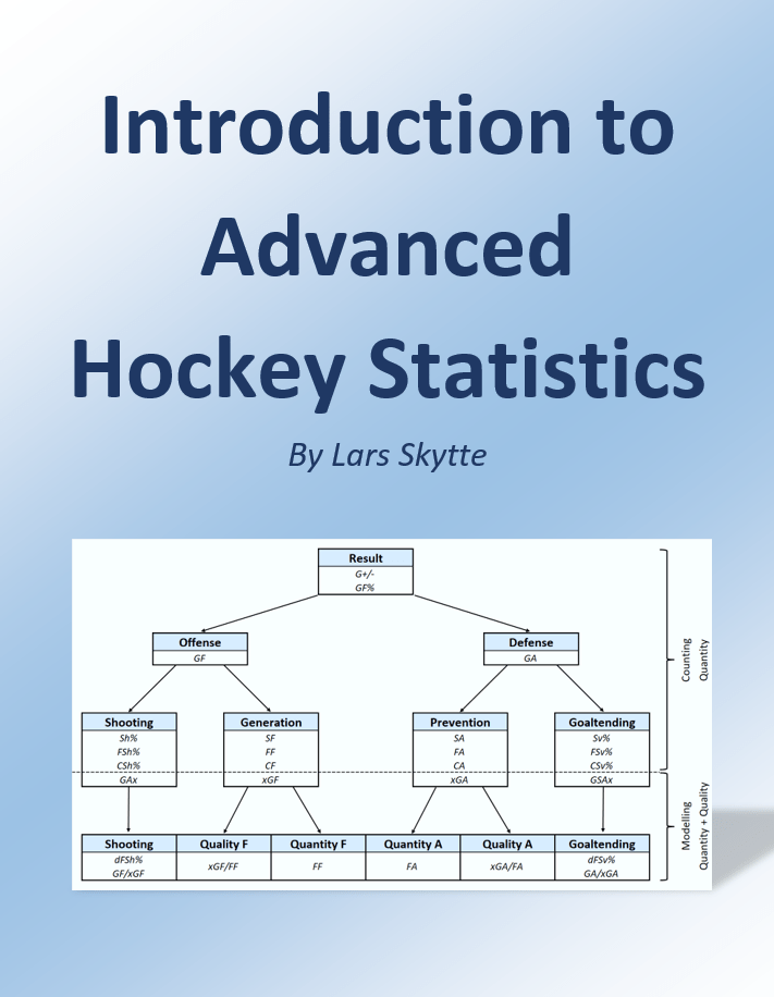
2. Shot statistics

Most statistics in hockey is based on shots. So, that will naturally be the focus in the first chapter. I think the best way to describe shot statistics is through a shot hierarchy. At the top you have the result, and then you can use shot data to describe how the result occurred.

2.1 – Shot Hierarchy

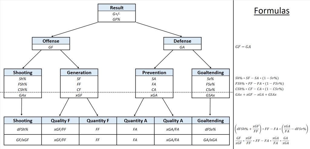
I will start off by showing the entire hierarchy in a single chart, and then I will walk you through each component step by step.

Here’s the shot chart:

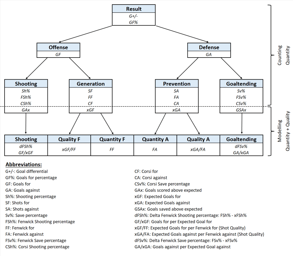
Result:

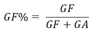
The ultimate goal in hockey is to score more goals than your opponent, so you can define the result as either goal differential (G+/-) or goals for percentage (GF%).

Clearly, the result is the end goal. All other analysis is either designed to describe how the results occurred or to predict future results.

Offense vs. Defense:

Statistically offense is defined as goals for and defense is defined as goals against. This makes sense statistically because it allows us to easily quantify offense and defense.

However, it’s not how I (as a coach) would define offense and defense. In my definition, offense is the play when the team has possession of the puck and defense is the play when the opposition has possession of the puck. It’s important to understand the difference!

Statistically, a team can play good defensive hockey by playing good possession hockey. If you possess the puck, you can’t get scored on.

Say, a player in the offensive zone makes a high risk play which results in a breakaway and a goal against. Statistically speaking it’s a bad defensive play, but intuitively it’s a bad offensive play that leads to the goal against.

Shooting and Goaltending (Counting stats):

In the NHL data there are 4 types of shot events:

1. Goal
2. Shot (on goal)
3. Miss
4. Block

These shot types are then categorized in 4 statistical groups. It’s a bit confusing that the event “shot” doesn’t include goals, but the statistic “shot” does:

1. Goals
2. Shots: Goals + Shots
3. Fenwick: Goals + Shots + Misses
4. Corsi: Goals + Shots + Misses + Blocks

The naming here is somewhat stupid, but other that that it’s pretty straight forward. Corsi simply means all shot attempts (SAT), fenwick means all unblocked shot attempts (USAT), shot means shot attempts that hits the net (including goals) and goals just mean goals.

Goals, shots, fenwick and corsi are what we call simple counting stats. This means that you’re simply counting the number of shot attempts. There’s no modelling involved.

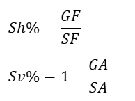
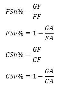
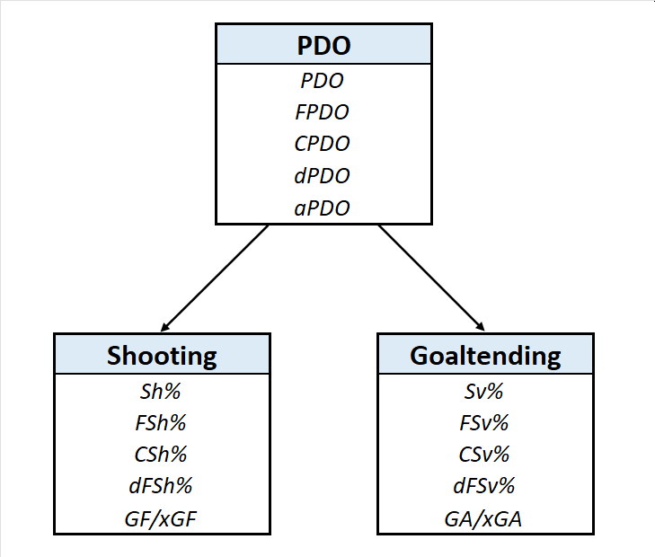
If we look at the shot hierarchy, we see that offense and defense is split into shooting/generation and goaltending/prevention respectively. At first, we’re going to focus on shooting and goaltending. You would typically define shooting as Sh% and goaltending as Sv%:

However, you could also define shooting/goaltending based on fenwick or corsi:

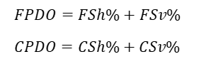
If you combine shooting and goaltending, you get regular PDO:

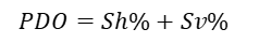
This is the format you would see on stats sites, but you could also calculate PDO based on fenwick or corsi:

The reason you look at PDO, is because shooting and goaltending are less predictable than generation and prevention (More on this in chapter 3). This means that there’s a higher variance in shooting and goaltending stats.

So, if the PDO is a lot higher or lower than 100%, there’s a good chance the results are unsustainable. You often hear that PDO will regress towards 100% over time, but this isn’t necessarily true – Some teams have better than average goaltenders and shooters.

Over time the PDO should regress towards the true quality of the shooters/goaltenders.

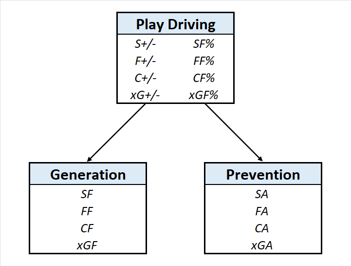
Generation and Prevention (Counting stats):

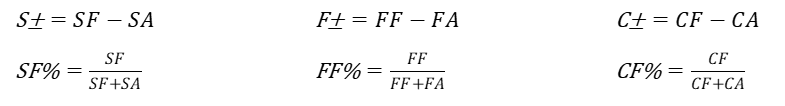
Now, we will turn our attention to shot generation and shot prevention. This is simply the number of shots you generate and the number of shots you allow. Prevention means allowing as few shots as possible.

You often talk about shot differentials. The goal is to generate more shots than you allow. You can either look at normal differentials or you can look at percentages:

The difference between shots generated and shots allowed is called play driving. So, when someone talks about play driving, they are likely referring to CF% or xGF% (more on that below).

Shooting and Goaltending (Modelling):

Until this point, we’ve only focused on counting stats. Let’s now look at modelling stats (the stats below the dashed line in the shot hierarchy image).

What do I mean by a modelling stat? All the counting stats consists of just a single variable that you simply count. When we’re building a model, we combine multiple variables and parameters.

All the modelling stats in the shot hierarchy are connected to expected goals. So, it’s very important to understand what xG is.

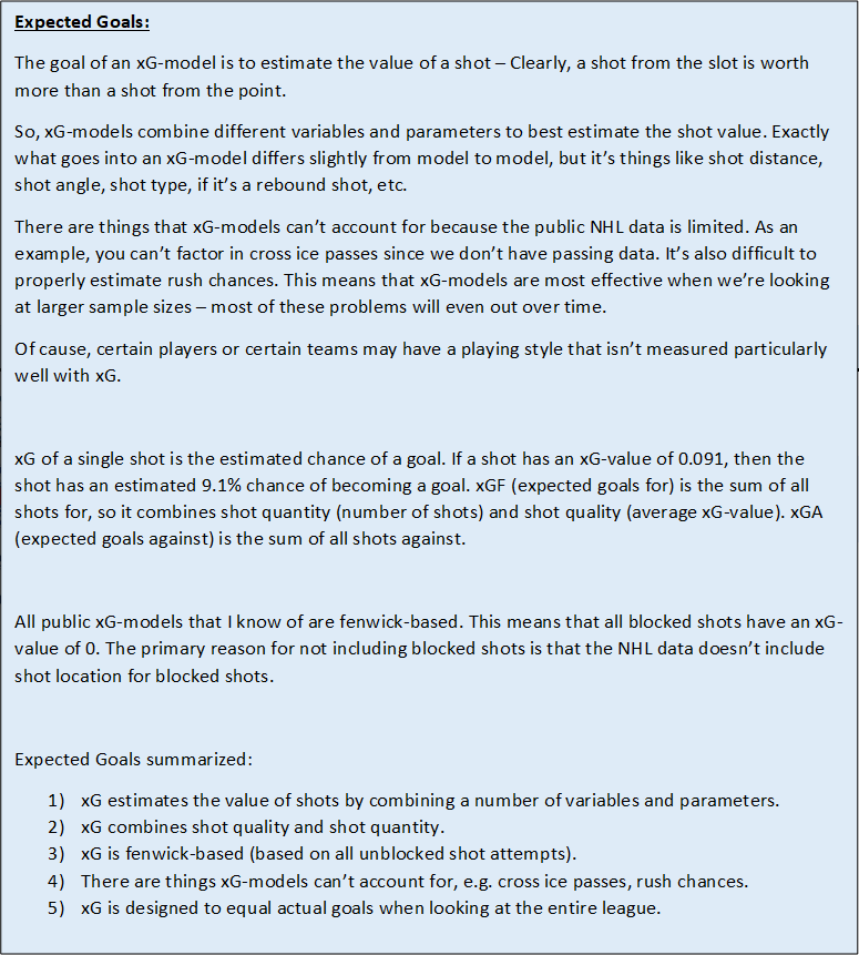
Now that we have talked about expected goals, we can discuss the more advanced shooting and goaltender stats. In this paragraph we will go through 3 different ways of measuring shooting and goaltending:

1. GAx and GSAx
2. dFSh% and dFSv%
3. GF/xGF and GA/xGA

Let’s go through them chronologically. GAx and GSAx is simply goals scored above expected and goals saved above expected respectively:

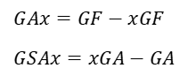
This is a way to measure the total shooting/goaltending impact. How many goals have been scored/saved above expected?

Sometimes we’re interested in measuring performance rather than impact. And what do I mean by that? If two goaltenders perform at the same level, but one of them is a starter and the other is a backup, then naturally the starter will have the greatest impact.

You can measure performance a few different ways. You could measure impact per 60 minutes, you could measure impact per shot, or you could measure impact per expected goal.

For goaltending and shooting it’s common to measure performance as impact per shot. That’s also what we do when we use Sh% and Sv%.

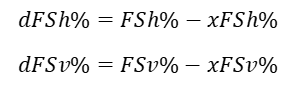
The advanced alternatives to Sh% and Sv% are dFSh% and dFSv%. These are defined as fenwick shooting percentage above expected and fenwick save percentage above expected:

It turns out that dFSh% is actually the same GAx per fenwick and dFSv% is the same as GSAx per fenwick:

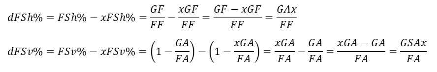
So, dFSh% and dFSv% are ways to measure shooting and goaltending performance as impact per fenwick (unblocked shot attempt). This is often how you see goaltender performance being measured.

The 3^rd option is to measure GF/xGF and GA/xGA. How many goals are scored/allowed per expected goal? Here we are measuring performance in regard to expected goals instead of fenwicks. If GF/xGF is above 1, you’re scoring more than expected. If GA/xGA is above 1, your goaltending is below expected.

It’s preferable to measure performance in regard to xG instead of fenwicks, because it’s fairer. Say, two above average goaltenders have the same GSAx and they have faced the same number of shots (FA). One of them (goaltender A) has faced more difficult shots (higher xGA). The two goaltenders have performed equally well if we use dFSv% (they faced the same number of shots). But if we use GA/xGA then goaltender B has the best performance. He has the same impact (GSAx) on a smaller workload (xGA).

So, I think GF/xGF and GA/xGA are the best ways to measure shooting/goaltender performance… But dFSh% and dFSv% are the consensus metrics. In other words, you will need to understand both metrics.

Earlier we discussed PDO. This was a way to combine goaltending and shooting into one metric. We can obviously do something similar with the more advanced goaltender/shooting stats. Here’s how I would define delta-PDO or dPDO:

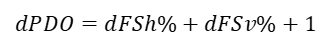
dPDO can be used the same way regular PDO, but it’s a better metric since it includes shot quality.

Alternatively, we could define analytics-PDO or aPDO as:

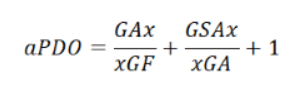
This would be my preferred metric for combined goaltending and shooting.

You won’t find dPDO or aPDO anywhere. People are still using regular PDO, but I consider these metrics better. So, help spread the word.

Generation and Prevention (Modelling):

The final part of the shot hierarchy is the advanced generation/prevention part. Generation is simply xGF, whereas prevention is xGA. Unlike the counting stats, these metrics combine shot quantity and shot quality. In fact, you can split up generation/prevention into quality and quantity.

Shot quality is defined as xG per fenwick – the average shot-value. Shot quantity is just the total number of shots. We’re using fenwicks, because xG-models are fenwick-based.

Like mentioned earlier, the combination generation and prevention is called play driving:

2.2 – Shot Formulas

In this paragraph of the chapter, we will look at shot formulas. It’s not necessary to understand all of this, but it should help give you an understanding of how each metric is connected.

Here’s the formulas connected to each step of the shot hierarchy. All the formulas are equal to the goal differential (G+/-), so it’s a way to calculate the result.

On the next few pages, I will show all the calculations behind the formulas. If you’re not interested in knowing how the formulas have come about, you can just skip this part and go the “Shot Tracking” paragraph.

Shots:

For the rest of you, we will start off by looking at shots. I start by looking at goals for (GF), then goals against (GA) and lastly I combine the two.

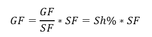
The first step is to just divide by SF and multiply SF, and since GF/SF is the same Sh% we get:

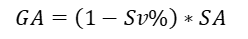
For GA it’s a bit more complicated. We start by adding and subtracting SA. Then we divide and multiply by SA, and get:

Since: Sv% = 1 – (GA/SA) , we must get:

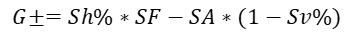
Finally, we can combine GF and GA:

Fenwick and Corsi:

The calculations for fenwick and corsi are exactly the same, so I will just show the results:

xG – (GAx and GSAx):

The next calculation is super simple. We just add and subtract xGF and xGA:

And since: GAx = GF – xGF and GSAx = xGA – GA, we get:

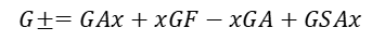
This could also be written as:

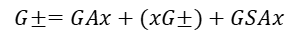
So, shooting impact + play driving + goaltender impact equals result! This is a good thing to remember.

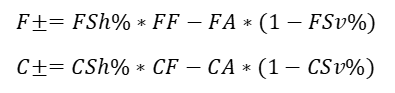
xG – (dFSh% and dFSv%):

In the next formula, we start by adding and subtracting xGF. Then we divide and multiply by fenwicks for (FF):

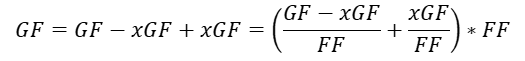
Since: GAx = GF – xGF and GAx/FA = dFSh%, we get:

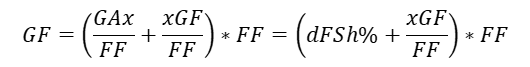
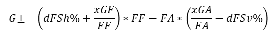
For GA the process is the same: We add and subtract xGA and then we divide and multiply by FA:

When we combine GF and GA, we get:

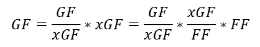
xG – (GF/xGF and GA/xGA):

In the final formula we divide and multiply xGF and then we divide and multiply by FF:

We do the same for GA:

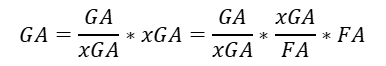
And combined it gives:

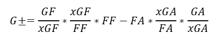
So, results equal:

shooting * shot quality for * shot quantity for – shot quantity against * shot quality against * goaltending

That’s beautiful!

2.3 – Shot Tracking

Until now we have discussed the different shot metrics and how they are connected. In the final paragraph of this chapter, I would like to talk about the data itself. How is it tracked and are there any pitfalls?

How are shots tracked?:

All public NHL shot data is manually tracked. I expect some of the tracking to become automated in the very near future, but for now everything is manually tracked.

This means that the data isn’t flawless, and we need to be aware of this. All data is tracked by the home team. When you track data in this fashion, it’s very likely that you end up with data differences from arena to arena. This could skew the home data for some teams.

From a scientific standpoint you should randomize the trackers, so that potential differences would even out with a large enough sample size. As it is now, those differences will accumulate onto specific teams.

Accuracy vs. Precision:

This leads us to a discussion about accuracy versus precision. High accuracy means the average of the datapoints is correct. There might be mistakes, but those mistakes will even out, and the average will be correct. High precision means the datapoints are collected the exact same way, so they will always be close. However, if the accuracy is low, then all the datapoints will be wrong.

Accuracy and precision are illustrated in the following image:

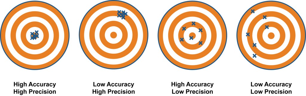
How does this relate to NHL data? Since all data is tracked manually, we can’t expect high precision. The same shot will be tracked differently – this is unavoidable. The hope is that on average the shot is tracked correctly (high accuracy). If the data has a high accuracy, then all our interpretations will be fine, for as long as we’re looking at a sufficiently large sample size. However, if the accuracy is low, then we have problems.

I won’t go into details in this book, but there are indications that shots in some arenas are tracked too close to the net, and in other arenas shots are tracked too far away from the net. This skews the xG data in those arenas. You can read about it in this article:

Indications that shot location data is flawed – Depends on where games are being played – Hockey-Statistics

When the data has a low accuracy, we need to calibrate the data, so that the average is correct. Some xG-models adjusts for rink bias (calibrates the model) and some xG-models don’t. This is beyond the content of this book, but it’s something to be aware of – especially when home numbers differ drastically from away numbers.

For more information about Accuracy and Precision, I recommend reading this article by Garret Hohl:

https://hockey-graphs.com/2021/03/16/behind-the-numbers-paretos-principle-power-law-distribution-and-when-tracking-data-does-not-matter/amp/

2.4 – Summary

– Shot events can be: A Goal, a Shot, a Miss or a Block.

– Fenwick means all unblocked shot attempts: Goals + Shots + Misses.

– Corsi means all shot attempts: Goals + Shots + Misses + Blocks.

– Expected Goals is an estimate of shot value, and all xG-models are based on fenwicks.

– The shot hierarchy explains the results via shot metrics.

– Impact is measured in totals, whereas performance is measured in rates (Impact per 60, fenwick or xG)

– PDO metrics combine goaltending and shooting.

– Play driving combines generation and prevention.

– High accuracy means the average is correct, even if the individual datapoints aren’t correct.

– High precision means the datapoints are always collected the same, even if it’s incorrect.