
Abstract:
In the previous article I laid the groundwork for my game projection model. Now I will use the actual starting lineups and add in season adjustments using the ELO ranking principle.
The data used in this article is from the 2016/2017 season to the 2019/2020 season.
Finding the starting lineups:
I used Evolving-Hockey’s Shift Query to find the lineups. I only used data from the first period, so that I would get the right starting goaltender. In the rare case where both goalies played in the first period, I can’t determine who the starter was, so I’m just using an average of the two. On average it happens around once per team per year.
Adding the variables:
Now I have the lineups for every game in the past 4 seasons, and I can add the variables. The spreadsheet is set up so I can easily add or change the variables used in the model.
Today I’m using 4 variables – the same I used in the season projection model: Skater_p-sGAA, Average Skater_Age, Average Skater_pTOI (weighted TOI the previous 3 seasons) and GK_p-sGAA.
At first, I’m just adding player projections: Skater_p-sGAA and GK_p-sGAA. The process is the same as in the last article, so first I will find the team strength (Win%):
Win% = 0.5 + (Skater_p-sGAA + GK_p-sGAA)*x
I’m obviously also adjusting for home ice advantage, and so I can find the Win probability and the projected point total for the game:
Win probability = Win%/(Win%+Win%(opposition)
pPoints = Win probability * 2.228
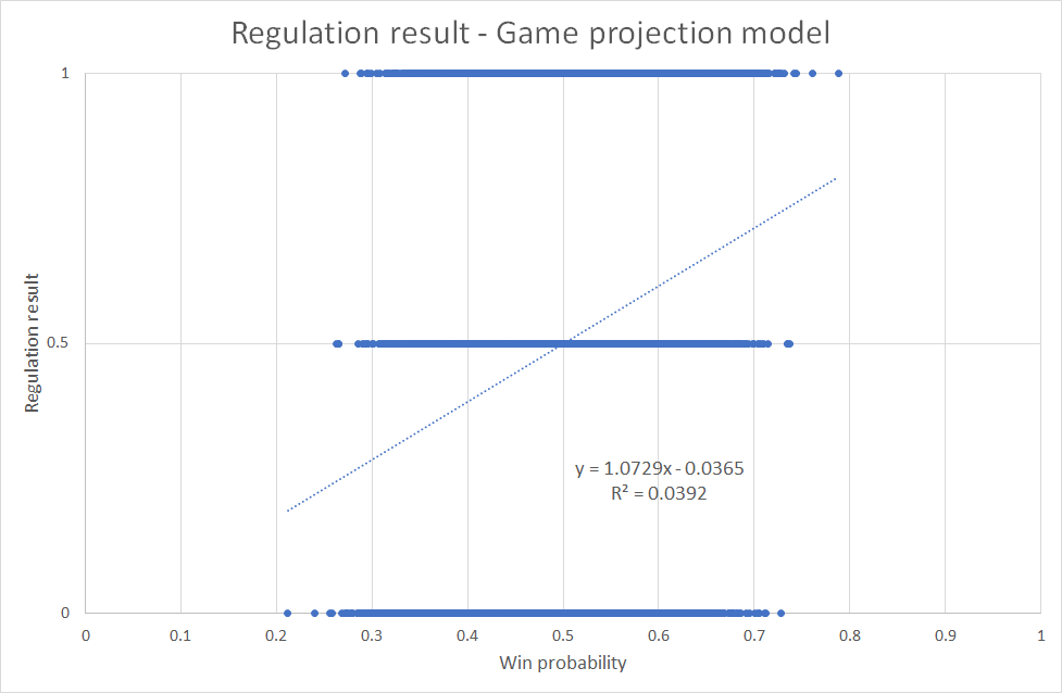
Last time I used x=0.0036, because then the season projection model equaled the game projection model. This time I will re-determine x. There’re a few different ways I can do this. I want the model to project game results as well as possible, so I will refine x towards giving the best single game results. I’ve decided to use regulation results, since overtime and shootout wins are more random. A win is worth 1, a tie is worth 0.5 and a loss is worth 0.
Then I can draw the regulation result as a function of the win probability, and find the x value that gives the best correlation (R^2). The best correlation came with x=0.0059:
I went through the same process to determine the weight put on the Age and pTOI components. For clarification I used Age above league average and pTOI above league average. So, if the Age component is below 0 it means the average player on the team was younger than league average.
I found the best correlation when I multiplied the Age component with -4 and the pTOI component with 0.05:
0.5 + (Skater_p-sGAA + GK_p-sGAA – 4*Skater_Age + 0.05*Skater_pTOI)*0.0059
That gives us the following graph:

Discussion:
There are a few things worth mentioning at this point. I could’ve chosen to refine the data towards something else. It may be smarter to refine towards goal differential, so a big win is worth more than a narrow win. In the end I don’t think the difference is huge, and I would have to make an adjustment for empty net goals.
Regarding the variables, I plan to add more along the way, but this is a good starting point. It would be obvious to also add GK_Age and GK_pTOI to the equation. There are still no in-season adjustments. All the variables depend on preseason data alone, but I will get to that later on.
There’s also a case to be made for using rates (p-sGAA/pTOI) instead of totals. In the preseason projection it’s a good assumption that players play the same role from year to year. However, in the game projections I’m using the actual lineups, so I don’t have to estimate ice time to the same extent. Using rates would complicate things quite a bit, but it’s something I will test out at some point.
Interpreting the data so far:
It’s time to compare the season projection model with the game projection model. We should expect better results, since we’ve added more information. The season projection is based solely on opining night rosters, while the game projections include game day lineups.
So, let’s start by comparing point projections. Beneath are the average point error between the projection and the actual results:
Season projection model:
| Season | Average error |
|---|---|
| 16-17 | 9.84 |
| 17-18 | 11.69 |
| 18-19 | 7.66 |
| 19-20 | 6.90 |
| total | 9.02 |
Game projection model:
| Season | Average error |
|---|---|
| 16-17 | 9.60 |
| 17-18 | 11.58 |
| 18-19 | 8.42 |
| 19-20 | 6.53 |
| total | 9.03 |
It’s a bit concerning that the game projection model doesn’t project point total better than the season projection model. It’s important to remember that neither model make any in season adjustments based on performance, so perhaps the results aren’t too surprising. Also, the game projection model is refined towards projecting single games, not season results.
So, let’s turn our attention towards game projections instead. We can visualize the difference between the two models by showing the regulation result (win, loss, draw) as a function of win probability – the same graph used to refine the data:
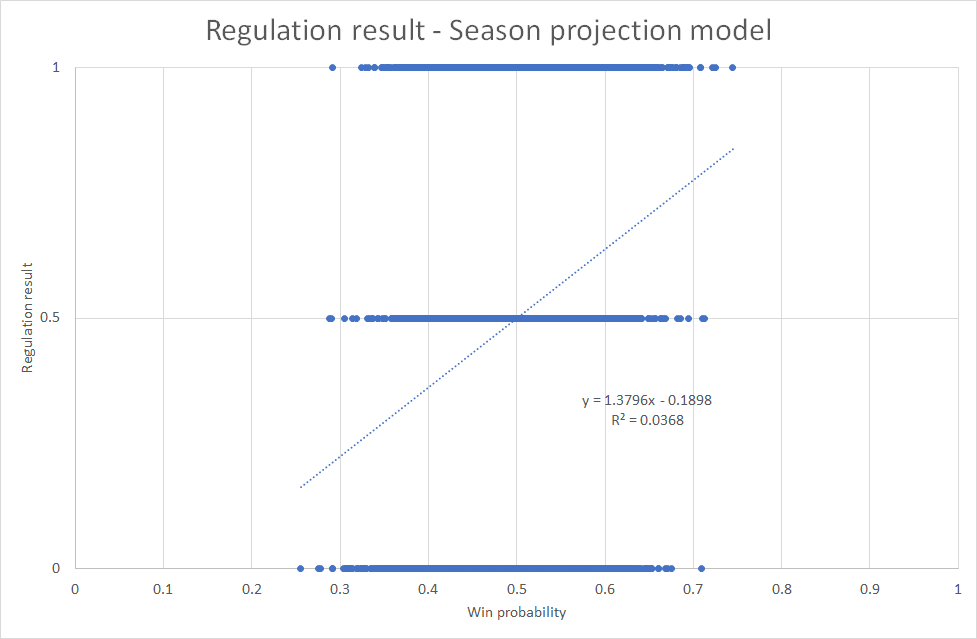
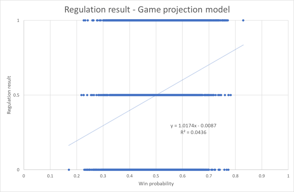
The game projection model clearly projects results better than the season model (R^2 is higher). It’s also more “aggressive” in the projections. The biggest favorite in the season projection model was a 75/25 favorite. In the game projection model, the biggest favorite was an 83/17 favorite.
We could also compare the results to win probability in table form:
Season projection model:
| Probability | GP | Wins | Result |
|---|---|---|---|
| 70+ | 19 | 18 | 94.7 |
| 65-70 | 130 | 95 | 73.1 |
| 60-65 | 602 | 400 | 66.4 |
| 55-60 | 1683 | 983 | 58.4 |
| 50-55 | 2420 | 1283 | 53.0 |
| Total | 4854 | 2779 | 57.3 |
Game projection model:
| Probability | GP | Wins | Result |
|---|---|---|---|
| 75+ | 22 | 18 | 81.8 |
| 70-75 | 80 | 66 | 82.5 |
| 65-70 | 349 | 236 | 67.6 |
| 60-65 | 892 | 551 | 61.8 |
| 55-60 | 1576 | 918 | 58.2 |
| 50-55 | 1935 | 1020 | 52.7 |
| Total | 4854 | 2809 | 57.9 |
Adding ELO adjustments:
The next and final step is to add in season adjustments. In theory it would be nice to use sGAA to adjust the team strength. That’s not possible though since GAR/xGAR (the basis of sGAA) can’t be found for individual games. I will instead use the principal from ELO rankings. Winning as an underdog is worth more than winning as a favorite.
The new team strength (Win%) after a game is calculated this way:
Win%(new) = Win%(old) + k*(Result – Win probability)
I’m using regulation result in this calculation. The k variable determines how aggressive the adjustments are. I have refined k using the same approach as I did above, and the best correlation is when k=0.017. Here’s the graph:

Now the model adjusts based on results, so we should expect a better point projection. If the model was wrong in the preseason it will self-adjust. Here’s the average point error in the ELO adjusted model:
| Season | Average error |
|---|---|
| 16-17 | 6.33 |
| 17-18 | 8.23 |
| 18-19 | 6.39 |
| 19-20 | 4.57 |
| total | 6.38 |
What’s perhaps more interesting is seeing how the ELO-adjustments affect the game projections.
| Probability | GP | Wins | Result |
|---|---|---|---|
| 75+ | 48 | 42 | 87.5 |
| 70-75 | 124 | 84 | 67.7 |
| 65-70 | 374 | 257 | 68.7 |
| 60-65 | 946 | 600 | 63.4 |
| 55-60 | 1517 | 898 | 59.2 |
| 50-55 | 1845 | 943 | 51.1 |
| Total | 4854 | 2824 | 58.2 |
The game probabilities match the game results quite well. The goal is to have a model that’s aggressive in its predictions, but still have the correct probabilities.
As always it’s worth comparing the findings to Dom Luszcyszyn’s results. I could only find his game probabilities from the past 3 seasons, so that will be the basis of the comparison. Here’s Dom’s results:
| Probability | GP | Wins | Result |
|---|---|---|---|
| 75+ | 26 | 22 | 84.6 |
| 70-75 | 100 | 66 | 66.0 |
| 65-70 | 334 | 225 | 67.4 |
| 60-65 | 721 | 444 | 61.6 |
| 55-60 | 1101 | 675 | 61.3 |
| 50-55 | 1341 | 665 | 49.6 |
| Total | 3623 | 2097 | 57.9 |
And here’s the results from my model the last 3 years:
| Probability | GP | Wins | Result |
|---|---|---|---|
| 75+ | 46 | 40 | 87.0 |
| 70-75 | 98 | 66 | 67.3 |
| 65-70 | 278 | 185 | 66.5 |
| 60-65 | 709 | 447 | 63.0 |
| 55-60 | 1120 | 660 | 58.9 |
| 50-55 | 1373 | 709 | 51.6 |
| Total | 3624 | 2107 | 58.1 |
In terms of aggressiveness the two models are very similar – same number of games in each span. My model is more correct in the predictions though.
Points vs. pPoints:
When the new season starts (knock on wood), I plan to make points vs. projected points graphs. This way you can easily see if a team is under- or over-performing compared to the model.
Here I have also added the projected points without any ELO adjustments. Just to show how they work. Here’s the T.B 18/19 team. A team that was really consistent and outperformed the model by a large margin:
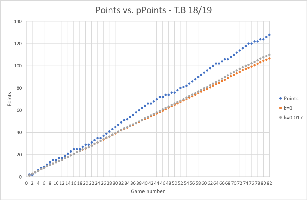
The ELO adjustments here seem pretty minor, but the goal isn’t to end up at right point total. The goal is to correct towards the right slope.
Here’s the BUF 18/19 team. An up and down team:
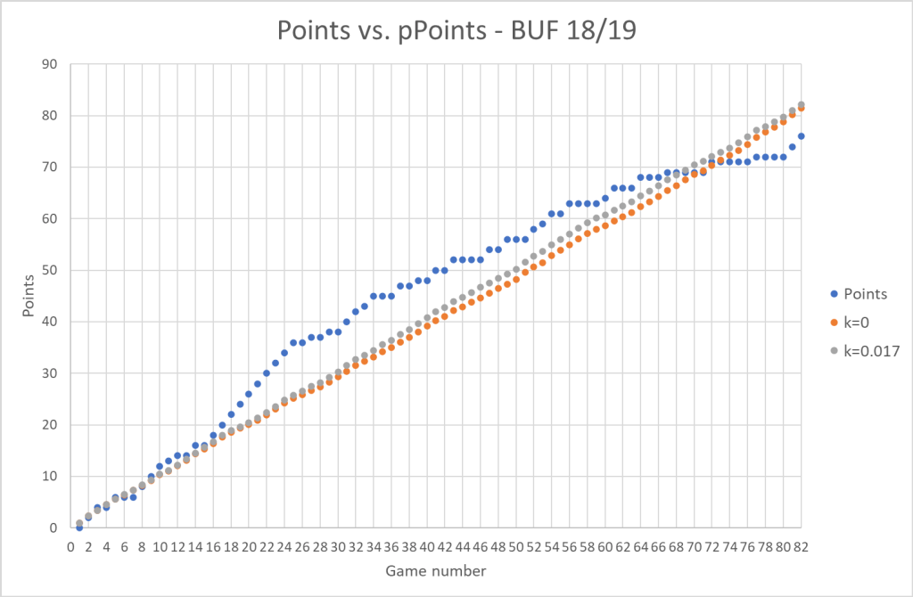
The model was good until the 10 game win streak.
Perspective:
There’s still a lot of improvements I can make to the model, but I’m really pleased with the overall process. All the workbooks are set up in a way, where I can easily change or add to the model. In other words, I like the thought process behind the model. Now I just need to improve the data input.
First step is to re-calculate the sGAA and p-sGAA. Evolving-Hockey has updated their GAR and xGAR models, so I will have to do the same. I doubt that leads to any huge changes.
Next, I will rethink the variables. Adding GK_Age and GK_pTOI seem obvious, but I might do something else as well. I still think it’s possible to improve the goaltender projections (GK_p-sGAA), but I will probably leave them as they are for now.
The plan is to do season previews once the schedule is announced, and then have daily game projections based on the above model.
Data from www.Evolving-Hockey.com, www.naturalstattrick.com and www.theathletic.com
